True Measures

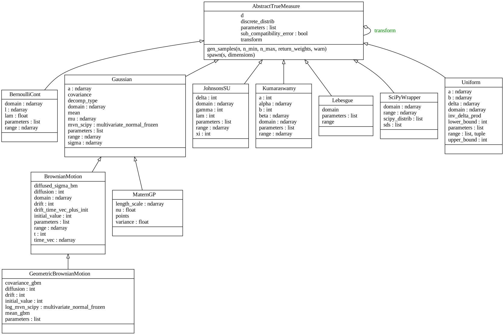
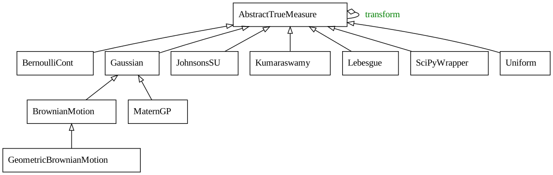
UML Overview

AbstractTrueMeasure

Bases: object

Source code in qmcpy/true_measure/abstract_true_measure.py

def __init__(self):
    prefix = "A concrete implementation of TrueMeasure must have "
    if not hasattr(self, "domain"):
        raise ParameterError(
            prefix
            + "self.domain, 2xd ndarray of domain lower bounds (first col) and upper bounds (second col)"
        )
    if not hasattr(self, "range"):
        raise ParameterError(
            prefix
            + "self.range, 2xd ndarray of range lower bounds (first col) and upper bounds (second col)"
        )
    if not hasattr(self, "parameters"):
        self.parameters = []

__call__

__call__(n=None, n_min=None, n_max=None, return_weights=False, warn=True)

• If just n is supplied, generate samples from the sequence at indices 0,...,n-1.
• If n_min and n_max are supplied, generate samples from the sequence at indices n_min,...,n_max-1.
• If n and n_min are supplied, then generate samples from the sequence at indices n,...,n_min-1.

Parameters:

Name	Type	Description	Default
n	Union[None, int]	Number of points to generate.	None
n_min	Union[None, int]	Starting index of sequence.	None
n_max	Union[None, int]	Final index of sequence.	None
return_weights	bool	If True, return weights as well	False
warn	bool	If False, disable warnings when generating samples.	True

Returns:

Name	Type	Description
t	ndarray	Samples from the sequence. If replications is None then this will be of size (n_max-n_min) \(\times\) dimension If replications is a positive int, then t will be of size replications \(\times\) (n_max-n_min) \(\times\) dimension
weights	ndarray	Only returned when return_weights=True. The Jacobian weights for the transformation

Source code in qmcpy/true_measure/abstract_true_measure.py

def __call__(self, n=None, n_min=None, n_max=None, return_weights=False, warn=True):
    r"""
    - If just `n` is supplied, generate samples from the sequence at indices 0,...,`n`-1.
    - If `n_min` and `n_max` are supplied, generate samples from the sequence at indices `n_min`,...,`n_max`-1.
    - If `n` and `n_min` are supplied, then generate samples from the sequence at indices `n`,...,`n_min`-1.

    Args:
        n (Union[None, int]): Number of points to generate.
        n_min (Union[None, int]): Starting index of sequence.
        n_max (Union[None, int]): Final index of sequence.
        return_weights (bool): If `True`, return `weights` as well
        warn (bool): If `False`, disable warnings when generating samples.

    Returns:
        t (np.ndarray): Samples from the sequence.

            - If `replications` is `None` then this will be of size (`n_max`-`n_min`) $\times$ `dimension`
            - If `replications` is a positive int, then `t` will be of size `replications` $\times$ (`n_max`-`n_min`) $\times$ `dimension`
        weights (np.ndarray): Only returned when `return_weights=True`. The Jacobian weights for the transformation
    """
    return self.gen_samples(
        n=n, n_min=n_min, n_max=n_max, return_weights=return_weights, warn=warn
    )

spawn

spawn(s=1, dimensions=None)

Spawn new instances of the current true measure but with new seeds and dimensions. Used by multi-level QMC algorithms which require different seeds and dimensions on each level.

Note

Use replications instead of using spawn when possible, e.g., when spawning copies which all have the same dimension.

Parameters:

Name	Type	Description	Default
s	int	Number of copies to spawn	1
dimensions	ndarray	Length s array of dimensions for each copy. Defaults to the current dimension.	None

Returns:

Name	Type	Description
spawned_true_measures	list	True measure with new seeds and dimensions.

Source code in qmcpy/true_measure/abstract_true_measure.py

def spawn(self, s=1, dimensions=None):
    r"""
    Spawn new instances of the current true measure but with new seeds and dimensions.
    Used by multi-level QMC algorithms which require different seeds and dimensions on each level.

    Note:
        Use `replications` instead of using `spawn` when possible, e.g., when spawning copies which all have the same dimension.

    Args:
        s (int): Number of copies to spawn
        dimensions (np.ndarray): Length `s` array of dimensions for each copy. Defaults to the current dimension.

    Returns:
        spawned_true_measures (list): True measure with new seeds and dimensions.
    """
    sampler = self.discrete_distrib if self.transform == self else self.transform
    sampler_spawns = sampler.spawn(s=s, dimensions=dimensions)
    spawned_true_measures = [None] * len(sampler_spawns)
    for i in range(s):
        spawned_true_measures[i] = self._spawn(
            sampler_spawns[i], sampler_spawns[i].d
        )
    return spawned_true_measures

SciPyWrapper

Bases: AbstractTrueMeasure

True measure that wraps SciPy style distributions.

This class keeps the original behavior of SciPyWrapper with independent 1D marginals and adds an optional "joint" mode for dependent distributions.

Examples:

Independent marginals from scipy.stats:

>>> import scipy.stats as stats
>>> tm = SciPyWrapper(
...     sampler=DigitalNetB2(3, seed=7),
...     scipy_distribs=[
...         stats.uniform(loc=1, scale=2),
...         stats.norm(loc=0, scale=1),
...         stats.gamma(a=5, loc=0, scale=2)])
>>> x = tm(2)
>>> x.shape
(2, 3)

Joint multivariate normal passed as a single object:

>>> mvn = stats.multivariate_normal(
...     mean=[0.0, 0.0],
...     cov=[[1.0, 0.8], [0.8, 1.0]])
>>> tm_joint = SciPyWrapper(DigitalNetB2(2, seed=7), mvn)
>>> tm_joint(2).shape
(2, 2)

2D Student t distribution (independent marginals):

>>> df = 5
>>> true_measure = SciPyWrapper(
...     sampler=DigitalNetB2(2, seed=13),
...     scipy_distribs=[
...         stats.t(df=df, loc=0.0, scale=1.0),
...         stats.t(df=df, loc=1.0, scale=2.0),
...     ],
... )
>>> xs = true_measure(4)
>>> xs.shape
(4, 2)

Parameters

sampler : AbstractDiscreteDistribution Low discrepancy or iid sampler in dimension d, living on [0,1)^d. scipy_distribs : One of the following:

- A single SciPy 1D continuous frozen distribution.
- A list of such frozen distributions (independent marginals).
- A custom 1D distribution object with ``ppf`` and ``pdf`` or
  ``logpdf`` methods.
- A joint object with:
    * ``transform(u)`` method
    * optional ``logpdf(x)`` method
    * ``dim`` or ``dimension`` attribute (otherwise ``sampler.d``).

Source code in qmcpy/true_measure/scipy_wrapper.py

def __init__(self, sampler, scipy_distribs):
    """
    Parameters
    ----------
    sampler : AbstractDiscreteDistribution
        Low discrepancy or iid sampler in dimension d, living on [0,1)^d.
    scipy_distribs :
        One of the following:

        - A single SciPy 1D continuous frozen distribution.
        - A list of such frozen distributions (independent marginals).
        - A custom 1D distribution object with ``ppf`` and ``pdf`` or
          ``logpdf`` methods.
        - A joint object with:
            * ``transform(u)`` method
            * optional ``logpdf(x)`` method
            * ``dim`` or ``dimension`` attribute (otherwise ``sampler.d``).
    """
    self.domain = np.array([[0.0, 1.0]])

    if not isinstance(sampler, AbstractDiscreteDistribution):
        if not (
            hasattr(sampler, "d")
            and hasattr(sampler, "gen_samples")
            and callable(sampler.gen_samples)
        ):
            raise ParameterError(
                "SciPyWrapper requires sampler be an AbstractDiscreteDistribution."
            )
    self._parse_sampler(sampler)

    # Remember what the user originally passed in so that _spawn can reuse it.
    self._user_distrib_arg = scipy_distribs

    # Flags and holders for the two modes.
    self._is_joint = False
    self._joint = None
    self._joint_has_logpdf = False
    self._warned_missing_pdf = False

    if self._looks_like_joint(scipy_distribs):
        # Configure joint mode.
        self._setup_joint(scipy_distribs)
    else:
        # Configure independent marginals mode.
        self._setup_marginals(scipy_distribs)

    super(SciPyWrapper, self).__init__()

Uniform

Bases: AbstractTrueMeasure

Uniform distribution, see https://en.wikipedia.org/wiki/Continuous_uniform_distribution.

Examples:

>>> true_measure = Uniform(DigitalNetB2(2,seed=7),lower_bound=[0,.5],upper_bound=[2,3])
>>> true_measure(4)
array([[1.44324713, 2.7873875 ],
       [0.32691107, 1.5741214 ],
       [1.97352511, 0.58590959],
       [0.8591331 , 1.89690854]])
>>> true_measure
Uniform (AbstractTrueMeasure)
    lower_bound     [0.  0.5]
    upper_bound     [2 3]

With independent replications

>>> x = Uniform(DigitalNetB2(3,seed=7,replications=2),lower_bound=[.25,.5,.75],upper_bound=[1.75,1.5,1.25])(4)
>>> x.shape
(2, 4, 3)
>>> x
array([[[0.61979915, 0.6821862 , 1.12366296],
        [1.27229355, 1.16169442, 0.9644598 ],
        [0.97209782, 1.29818233, 0.79100643],
        [1.62311988, 0.79520621, 1.13747905]],

       [[0.92315337, 1.35899604, 1.0027484 ],
        [1.05453886, 0.54353443, 0.91782473],
        [0.59821215, 0.79281506, 0.78420518],
        [1.37943573, 1.10241448, 1.13481488]]])

Parameters:

Name	Type	Description	Default
sampler	Union[AbstractDiscreteDistribution, AbstractTrueMeasure]	Either a discrete distribution from which to transform samples, or a true measure by which to compose a transform.	required
lower_bound	Union[float, ndarray]	Lower bound.	0
upper_bound	Union[float, ndarray]	Upper bound.	1

Source code in qmcpy/true_measure/uniform.py

def __init__(self, sampler, lower_bound=0, upper_bound=1):
    r"""
    Args:
        sampler (Union[AbstractDiscreteDistribution, AbstractTrueMeasure]): Either

            - a discrete distribution from which to transform samples, or
            - a true measure by which to compose a transform.
        lower_bound (Union[float, np.ndarray]): Lower bound.
        upper_bound (Union[float, np.ndarray]): Upper bound.
    """
    self.parameters = ["lower_bound", "upper_bound"]
    self.domain = np.array([[0, 1]])
    self._parse_sampler(sampler)
    self.lower_bound = lower_bound
    self.upper_bound = upper_bound
    if np.isscalar(self.lower_bound):
        lower_bound = np.tile(self.lower_bound, self.d)
    if np.isscalar(self.upper_bound):
        upper_bound = np.tile(self.upper_bound, self.d)
    self.a = np.array(lower_bound)
    self.b = np.array(upper_bound)
    if len(self.a) != self.d or len(self.b) != self.d:
        raise DimensionError(
            "upper bound and lower bound must be of length dimension"
        )
    self.delta = self.b - self.a
    self.inv_delta_prod = 1 / self.delta.prod()
    self.range = np.hstack(
        (self.a.reshape((self.d, 1)), self.b.reshape((self.d, 1)))
    )
    super(Uniform, self).__init__()
    assert self.a.shape == (self.d,) and self.b.shape == (self.d,)

Gaussian

Bases: AbstractTrueMeasure

Gaussian (Normal) distribution as described in https://en.wikipedia.org/wiki/Multivariate_normal_distribution.

Note

• Normal is an alias for Gaussian

Examples:

>>> true_measure = Gaussian(DigitalNetB2(2,seed=7),mean=[1,2],covariance=[[9,4],[4,5]])
>>> true_measure(4)
array([[ 3.83994612,  1.19097885],
       [-1.9727727 ,  0.49405353],
       [ 5.87242307,  8.41341485],
       [ 0.61222205,  1.48402653]])
>>> true_measure
Gaussian (AbstractTrueMeasure)
    mean            [1 2]
    covariance      [[9 4]
                     [4 5]]
    decomp_type     PCA

With independent replications

>>> x = Gaussian(DigitalNetB2(3,seed=7,replications=2),mean=0,covariance=3)(4)
>>> x.shape
(2, 4, 3)
>>> x
array([[[-1.18721904, -1.57108272,  1.15371635],
        [ 0.81749123,  0.72242445, -0.31025434],
        [-0.0807895 ,  1.44651585, -2.41042379],
        [ 2.38133494, -0.93225637,  1.30817519]],

       [[-0.22304017,  1.86337427,  0.02386568],
        [ 0.15807672, -2.96365385, -0.73502346],
        [-1.26753687, -0.94427848, -2.57683314],
        [ 1.1844196 ,  0.44964332,  1.27760936]]])

Parameters:

Name	Type	Description	Default
sampler	Union[AbstractDiscreteDistribution, AbstractTrueMeasure]	Either a discrete distribution from which to transform samples, or a true measure by which to compose a transform.	required
mean	Union[float, ndarray]	Mean vector.	0.0
covariance	Union[float, ndarray]	Covariance matrix. A float or vector will be expanded into a diagonal matrix.	1.0
decomp_type	str	Method for decomposition for covariance matrix. Options include 'PCA' for principal component analysis, or 'Cholesky' for cholesky decomposition.	'PCA'

Source code in qmcpy/true_measure/gaussian.py

def __init__(self, sampler, mean=0.0, covariance=1.0, decomp_type="PCA"):
    """
    Args:
        sampler (Union[AbstractDiscreteDistribution, AbstractTrueMeasure]): Either

            - a discrete distribution from which to transform samples, or
            - a true measure by which to compose a transform.
        mean (Union[float, np.ndarray]): Mean vector.
        covariance (Union[float, np.ndarray]): Covariance matrix. A float or vector will be expanded into a diagonal matrix.
        decomp_type (str): Method for decomposition for covariance matrix. Options include

            - `'PCA'` for principal component analysis, or
            - `'Cholesky'` for cholesky decomposition.
    """
    self.parameters = ["mean", "covariance", "decomp_type"]
    # default to transform from standard uniform
    self.domain = np.array([[0, 1]])
    self._parse_sampler(sampler)
    self._parse_gaussian_params(mean, covariance, decomp_type)
    self.range = np.array([[-np.inf, np.inf]])
    super(Gaussian, self).__init__()
    assert self.mu.shape == (self.d,) and self.a.shape == (self.d, self.d)

a property writable

a

Lazy-loaded decomposition matrix.

mvn_scipy property writable

mvn_scipy

Lazy-loaded scipy multivariate normal.

BrownianMotion

Bases: Gaussian

Brownian Motion as described in https://en.wikipedia.org/wiki/Brownian_motion. For a standard Brownian Motion \(W\) we define the Brownian Motion \(B\) with initial value \(B_0\), drift \(\gamma\), and diffusion \(\sigma^2\) to be

\[B(t) = B_0 + \gamma t + \sigma W(t).\]

Examples:

>>> true_measure = BrownianMotion(DigitalNetB2(4,seed=7),t_final=2,drift=2)
>>> true_measure(2)
array([[0.82189263, 2.7851793 , 3.60126805, 3.98054724],
       [0.2610643 , 0.06170064, 1.06448269, 2.30990767]])
>>> true_measure
BrownianMotion (AbstractTrueMeasure)
    time_vec        [0.5 1.  1.5 2. ]
    drift           2^(1)
    mean            [1. 2. 3. 4.]
    covariance      [[0.5 0.5 0.5 0.5]
                     [0.5 1.  1.  1. ]
                     [0.5 1.  1.5 1.5]
                     [0.5 1.  1.5 2. ]]
    decomp_type     PCA

With independent replications

>>> x = BrownianMotion(DigitalNetB2(3,seed=7,replications=2),t_final=2,drift=2)(4)
>>> x.shape
(2, 4, 3)
>>> x
array([[[0.66154685, 1.50620966, 3.52322901],
        [1.77064217, 3.32782204, 4.45013223],
        [1.33558688, 3.26017547, 3.40692337],
        [2.10317345, 3.78961839, 6.17948096]],

       [[1.77868019, 2.75347902, 3.41161419],
        [0.44891984, 2.53987304, 4.7224811 ],
        [0.23147948, 2.25289769, 3.00039101],
        [2.06762574, 3.21756319, 4.93375923]]])

Parameters:

Name	Type	Description	Default
sampler	Union[AbstractDiscreteDistribution, AbstractTrueMeasure]	Either a discrete distribution from which to transform samples, or a true measure by which to compose a transform.	required
t_final	float	End time.	1
initial_value	float	Initial value \(B_0\).	0
drift	int	Drift \(\gamma\).	0
diffusion	int	Diffusion \(\sigma^2\).	1
decomp_type	str	Method for decomposition for covariance matrix. Options include 'PCA' for principal component analysis, or 'Cholesky' for cholesky decomposition.	'PCA'
lazy_decomp	bool	If True, defer expensive matrix decomposition until needed.	True

Source code in qmcpy/true_measure/brownian_motion.py

def __init__(
    self,
    sampler,
    t_final=1,
    initial_value=0,
    drift=0,
    diffusion=1,
    decomp_type="PCA",
    lazy_decomp=True,
):
    r"""
    Args:
        sampler (Union[AbstractDiscreteDistribution, AbstractTrueMeasure]): Either

            - a discrete distribution from which to transform samples, or
            - a true measure by which to compose a transform.
        t_final (float): End time.
        initial_value (float): Initial value $B_0$.
        drift (int): Drift $\gamma$.
        diffusion (int): Diffusion $\sigma^2$.
        decomp_type (str): Method for decomposition for covariance matrix. Options include

            - `'PCA'` for principal component analysis, or
            - `'Cholesky'` for cholesky decomposition.
        lazy_decomp (bool): If True, defer expensive matrix decomposition until needed.
    """
    self.parameters = ["time_vec", "drift", "mean", "covariance", "decomp_type"]
    # default to transform from standard uniform
    self.domain = np.array([[0, 1]])
    self._parse_sampler(sampler)
    self.t = t_final  # exercise time
    self.initial_value = initial_value
    self.drift = drift
    self.diffusion = diffusion
    self.time_vec = np.linspace(self.t / self.d, self.t, self.d)  # evenly spaced
    self.diffused_sigma_bm = self.diffusion * np.minimum.outer(
        self.time_vec, self.time_vec
    )
    self.drift_time_vec_plus_init = (
        self.drift * self.time_vec + self.initial_value
    )  # mean
    self._parse_gaussian_params(
        self.drift_time_vec_plus_init,
        self.diffused_sigma_bm,
        decomp_type,
        lazy_decomp,
    )
    self.range = np.array([[-np.inf, np.inf]])
    super(Gaussian, self).__init__()

GeometricBrownianMotion

Bases: BrownianMotion

A Geometric Brownian Motion (GBM) with initial value \(S_0\), drift \(\gamma\), and diffusion \(\sigma^2\) is

\[\mathrm{GBM}(t) = S_0 \exp[(\gamma - \sigma^2/2) t + \sigma \mathrm{BM}(t)]\]

where BM is a Brownian Motion drift \(\gamma\) and diffusion \(\sigma^2\).

Examples:

>>> gbm = GeometricBrownianMotion(DigitalNetB2(4,seed=7), t_final=2, drift=0.1, diffusion=0.2)
>>> gbm.gen_samples(2)
array([[0.92343761, 1.42069027, 1.30851806, 0.99133819],
       [0.7185916 , 0.42028013, 0.42080335, 0.4696196 ]])
>>> gbm
GeometricBrownianMotion (AbstractTrueMeasure)
    time_vec        [0.5 1.  1.5 2. ]
    drift           0.100
    diffusion       0.200
    mean_gbm        [1.051 1.105 1.162 1.221]
    covariance_gbm  [[0.116 0.122 0.128 0.135]
                     [0.122 0.27  0.284 0.299]
                     [0.128 0.284 0.472 0.496]
                     [0.135 0.299 0.496 0.734]]
    decomp_type     PCA

Parameters:

Name	Type	Description	Default
sampler	DiscreteDistribution / TrueMeasure	A discrete distribution or true measure.	required
t_final	float	End time for the geometric Brownian motion, non-negative.	1
initial_value	float	Positive initial value of the process, \(S_0\).	1
drift	float	Drift coefficient \(\gamma\).	0
diffusion	float	Positive diffusion coefficient \(\sigma^2\), where \(\sigma\) is volatility.	1
decomp_type	str	Method of decomposition, either "PCA" or "Cholesky".	'PCA'
lazy_load	bool	If True, defer GBM-specific computations until needed.	True
lazy_decomp	bool	If True, defer expensive matrix decomposition until needed.	True

Source code in qmcpy/true_measure/geometric_brownian_motion.py

def __init__(
    self,
    sampler,
    t_final=1,
    initial_value=1,
    drift=0,
    diffusion=1,
    decomp_type="PCA",
    lazy_load=True,
    lazy_decomp=True,
):
    r"""
    Args:
        sampler (DiscreteDistribution/TrueMeasure): A discrete distribution or true measure.
        t_final (float): End time for the geometric Brownian motion, non-negative.
        initial_value (float): Positive initial value of the process, $S_0$.
        drift (float): Drift coefficient $\gamma$.
        diffusion (float): Positive diffusion coefficient $\sigma^2$, where $\sigma$ is volatility.
        decomp_type (str): Method of decomposition, either "PCA" or "Cholesky".
        lazy_load (bool): If True, defer GBM-specific computations until needed.
        lazy_decomp (bool): If True, defer expensive matrix decomposition until needed.
    """
    super().__init__(
        sampler,
        t_final=t_final,
        drift=0,
        diffusion=diffusion,
        decomp_type=decomp_type,
        lazy_decomp=lazy_decomp,
    )
    self.parameters = [
        "time_vec",
        "drift",
        "diffusion",
        "mean_gbm",
        "covariance_gbm",
        "decomp_type",
    ]
    self.initial_value = initial_value
    self.drift = drift
    self.diffusion = diffusion
    self.lazy_load = lazy_load
    self.lazy_decomp = lazy_decomp

    # Cache for lazy-loaded properties
    self._mean_gbm_cache = None
    self._covariance_gbm_cache = None
    self._log_mvn_scipy_cache = None

    # Large step optimization - use fast path for large problems
    self.large_step_threshold = 1000
    self.use_large_step_optimization = (
        len(self.time_vec) > self.large_step_threshold
    )

    # Validate input early (fast operation)
    self._validate_input()

    if not lazy_load:
        # Compute everything immediately for backwards compatibility
        self.mean_gbm = self._compute_gbm_mean()
        self.covariance_gbm = self._compute_gbm_covariance()
        self._setup_lognormal_distribution()

mean_gbm property writable

mean_gbm

Lazy-loaded GBM mean vector.

covariance_gbm property writable

covariance_gbm

Lazy-loaded GBM covariance matrix.

log_mvn_scipy property

log_mvn_scipy

Lazy-loaded scipy multivariate normal distribution.

gen_samples

gen_samples(n=None, n_min=None, n_max=None, return_weights=False, warn=True)

Generate GBM samples using the parent's transform pipeline.

Parameters:

Name	Type	Description	Default
n	int	number of samples to generate	None
n_min	int	minimum index of sequence	None
n_max	int	maximum index of sequence	None
return_weights	bool	whether to return Jacobian weights	False
warn	bool	whether to warn about sample generation	True

Returns:

Name	Type	Description
samples	Union[ndarray, tuple]	GBM samples, optionally with weights if return_weights=True

Source code in qmcpy/true_measure/geometric_brownian_motion.py

def gen_samples(
    self, n=None, n_min=None, n_max=None, return_weights=False, warn=True
) -> Union[ndarray, Tuple[ndarray, ndarray]]:
    """
    Generate GBM samples using the parent's transform pipeline.

    Args:
        n (int): number of samples to generate
        n_min (int): minimum index of sequence
        n_max (int): maximum index of sequence  
        return_weights (bool): whether to return Jacobian weights
        warn (bool): whether to warn about sample generation

    Returns:
        samples (Union[ndarray,tuple]): GBM samples, optionally with weights if return_weights=True
    """
    return super().gen_samples(n=n, n_min=n_min, n_max=n_max, return_weights=return_weights, warn=warn)

MaternGP

Bases: Gaussian

A Gaussian process with Matérn covariance kernel.

Examples:

>>> true_measure = MaternGP(DigitalNetB2(dimension=3,seed=7),points=np.linspace(0,1,3)[:,None],nu=3/2,length_scale=[3,4,5],variance=0.01,mean=np.array([.3,.4,.5]))
>>> true_measure(4)
array([[0.3515401 , 0.43083384, 0.51801119],
       [0.20272448, 0.31312011, 0.4241431 ],
       [0.40189226, 0.53502934, 0.63826677],
       [0.29943567, 0.38491661, 0.48296594]])
>>> true_measure
MaternGP (AbstractTrueMeasure)
    mean            [0.3 0.4 0.5]
    covariance      [[0.01  0.01  0.01 ]
                     [0.01  0.01  0.01 ]
                     [0.009 0.01  0.01 ]]
    decomp_type     PCA

With independent replications

>>> x = MaternGP(DigitalNetB2(dimension=3,seed=7,replications=2),points=np.linspace(0,1,3)[:,None],nu=3/2,length_scale=[3,4,5],variance=0.01,mean=np.array([.3,.4,.5]))(4)
>>> x.shape
(2, 4, 3)
>>> x
array([[[0.21490091, 0.33078241, 0.45151042],
        [0.35465127, 0.44705898, 0.53793358],
        [0.31091595, 0.39868187, 0.47660193],
        [0.42419919, 0.53572415, 0.64674883]],

       [[0.31010701, 0.38522001, 0.46670381],
        [0.27221177, 0.413546  , 0.54101758],
        [0.2147053 , 0.33293508, 0.43572791],
        [0.37343973, 0.46534628, 0.56356714]]])

References:

1. sklearn.gaussian_process.kernels.Matern.

2. https://en.wikipedia.org/wiki/Mat%C3%A9rn_covariance_function.

Parameters:

Name	Type	Description	Default
sampler	Union[AbstractDiscreteDistribution, AbstractTrueMeasure]	Either a discrete distribution from which to transform samples, or a true measure by which to compose a transform.	required
points	ndarray	The positions of points on a metric space. The array should have shape \((d,k)\) where \(d\) is the dimension of the sampler and \(k\) is the latent dimension.	required
nu	float	The "smoothness" of the MaternGP function, e.g., \(\nu = 1/2\) is equivalent to the absolute exponential kernel, \(\nu = 3/2\) implies a once-differentiable function, \(\nu = 5/2\) implies twice differentiability. as \(\nu \to \infty\) the kernel becomes equivalent to the RBF kernel, see sklearn.gaussian_process.kernels.RBF. Note that when \(\nu \notin \{1/2, 3/2, 5/2, \infty \}\) the kernel is around \(10\) times slower to evaluate.	1.5
length_scale	Union[float, ndarray]	Determines "peakiness", or how correlated two points are based on their distance.	1.0
variance	float	Global scaling factor.	1.0
mean	Union[float, ndarray]	Mean vector for multivariate Gaussian.	0.0
nugget	float	Positive nugget to add to diagonal.	1e-06
decomp_type	str	Method for decomposition for covariance matrix. Options include 'PCA' for principal component analysis, or 'Cholesky' for cholesky decomposition.	'PCA'

Source code in qmcpy/true_measure/matern_gp.py

def __init__(
    self,
    sampler,
    points,
    length_scale=1.0,
    nu=1.5,
    variance=1.0,
    mean=0.0,
    nugget=1e-6,
    decomp_type="PCA",
):
    r"""
    Args:
        sampler (Union[AbstractDiscreteDistribution, AbstractTrueMeasure]): Either

            - a discrete distribution from which to transform samples, or
            - a true measure by which to compose a transform.
        points (np.ndarray): The positions of points on a metric space. The array should have shape $(d,k)$ where $d$ is the dimension of the sampler and $k$ is the latent dimension.
        nu (float): The "smoothness" of the MaternGP function, e.g.,

            - $\nu = 1/2$ is equivalent to the absolute exponential kernel,
            - $\nu = 3/2$ implies a once-differentiable function,
            - $\nu = 5/2$ implies twice differentiability.
            - as $\nu \to \infty$ the kernel becomes equivalent to the RBF kernel, see [`sklearn.gaussian_process.kernels.RBF`](https://scikit-learn.org/stable/modules/generated/sklearn.gaussian_process.kernels.RBF.html#sklearn.gaussian_process.kernels.RBF).

            Note that when $\nu \notin \{1/2, 3/2, 5/2, \infty \}$ the kernel is around $10$ times slower to evaluate.
        length_scale (Union[float, np.ndarray]): Determines "peakiness", or how correlated two points are based on their distance.
        variance (float): Global scaling factor.
        mean (Union[float, np.ndarray]): Mean vector for multivariate `Gaussian`.
        nugget (float): Positive nugget to add to diagonal.
        decomp_type (str): Method for decomposition for covariance matrix. Options include

            - `'PCA'` for principal component analysis, or
            - `'Cholesky'` for cholesky decomposition.
    """
    if not (
        isinstance(sampler, AbstractDiscreteDistribution)
        or isinstance(sampler, AbstractTrueMeasure)
    ):
        raise ParameterError(
            "sampler input should either be an AbstractDiscreteDistribution or AbstractTrueMeasure."
        )
    if not (
        isinstance(points, np.ndarray) and (points.ndim == 1 or points.ndim == 2)
    ):
        raise ParameterError("points must be a one or two dimensional np.ndarray.")
    if points.ndim == 1:
        points = points[:, None]
    assert (
        points.ndim == 2 and points.shape[0] == sampler.d
    ), "points should be a two dimension array with the number of points equal to the dimension of the sampler"
    mean = np.array(mean)
    if mean.size == 1:
        mean = mean.item() * np.ones(sampler.d)
    assert mean.shape == (sampler.d,), "mean should be a length d vector"
    assert np.isscalar(nu) and nu > 0, "nu should be a positive scalar"
    length_scale = np.array(length_scale)
    if length_scale.size == 1:
        length_scale = length_scale.item() * np.ones(sampler.d)
    assert (
        length_scale.shape == (sampler.d,) and (length_scale > 0).all()
    ), "length_scale should be a vector with length equal to the dimension of the sampler"
    assert (
        np.isscalar(variance) and variance > 0
    ), "length_scale should be a positive scalar"
    assert np.isscalar(nugget) and nugget > 0, "nugget should be a positive scalar"
    self.points = points
    self.length_scale = length_scale
    self.nu = nu
    self.variance = variance
    dists = np.linalg.norm(
        points[..., :, None, :] - points[..., None, :, :], axis=-1
    )
    if nu == 1 / 2:
        covariance = np.exp(-dists / self.length_scale)
    elif nu == 3 / 2:
        covariance = (1 + np.sqrt(3) * dists / self.length_scale) * np.exp(
            -np.sqrt(3) * dists / self.length_scale
        )
    elif nu == 5 / 2:
        covariance = (
            1
            + np.sqrt(5) * dists / self.length_scale
            + 5 * dists**2 / (3 * self.length_scale**2)
        ) * np.exp(-np.sqrt(5) * dists / self.length_scale)
    elif nu == np.inf:
        covariance = np.exp(-(dists**2) / (2 * self.length_scale**2))
    else:
        k = np.sqrt(2 * nu) * dists / self.length_scale
        covariance = 2 ** (1 - nu) / gamma(nu) * k**nu * kv(nu, k)
    covariance = variance * covariance + nugget * np.eye(sampler.d)
    super().__init__(
        sampler, mean=mean, covariance=covariance, decomp_type=decomp_type
    )

Lebesgue

Bases: AbstractTrueMeasure

Lebesgue measure as described in https://en.wikipedia.org/wiki/Lebesgue_measure.

Examples:

>>> Lebesgue(Gaussian(DigitalNetB2(2,seed=7)))
Lebesgue (AbstractTrueMeasure)
    transform       Gaussian (AbstractTrueMeasure)
                        mean            0
                        covariance      1
                        decomp_type     PCA
>>> Lebesgue(Uniform(DigitalNetB2(2,seed=7)))
Lebesgue (AbstractTrueMeasure)
    transform       Uniform (AbstractTrueMeasure)
                        lower_bound     0
                        upper_bound     1

Parameters:

Name	Type	Description	Default
sampler	AbstractTrueMeasure	A true measure by which to compose a transform.	required

Source code in qmcpy/true_measure/lebesgue.py

def __init__(self, sampler):
    r"""
    Args:
        sampler (AbstractTrueMeasure): A true measure by which to compose a transform.
    """
    self.parameters = []
    if not isinstance(sampler, AbstractTrueMeasure):
        raise ParameterError(
            "Lebesgue sampler must be an AbstractTrueMeasure by which to transform samples."
        )
    self.domain = (
        sampler.range
    )  # hack to make sure Lebesgue is compatible with any transform
    self.range = sampler.range
    self._parse_sampler(sampler)
    super(Lebesgue, self).__init__()

BernoulliCont

Bases: AbstractTrueMeasure

Continuous Bernoulli distribution with independent marginals as described in https://en.wikipedia.org/wiki/Continuous_Bernoulli_distribution.

Examples:

>>> true_measure = BernoulliCont(DigitalNetB2(2,seed=7),lam=.2)
>>> true_measure(4)
array([[0.56205914, 0.83607872],
       [0.09433983, 0.28057299],
       [0.97190779, 0.01883497],
       [0.28050753, 0.39178506]])
>>> true_measure
BernoulliCont (AbstractTrueMeasure)
    lam             0.200

With independent replications

>>> x = BernoulliCont(DigitalNetB2(3,seed=7,replications=2),lam=[.25,.5,.75])(4)
>>> x.shape
(2, 4, 3)
>>> x
array([[[0.16343492, 0.1821862 , 0.83209443],
        [0.55140696, 0.66169442, 0.56381501],
        [0.35229402, 0.79818233, 0.13825119],
        [0.85773226, 0.29520621, 0.85203898]],

       [[0.32359293, 0.85899604, 0.63591945],
        [0.40278251, 0.04353443, 0.46749989],
        [0.1530438 , 0.29281506, 0.116725  ],
        [0.6345258 , 0.60241448, 0.84822692]]])

Parameters:

Name	Type	Description	Default
sampler	Union[AbstractDiscreteDistribution, AbstractTrueMeasure]	Either a discrete distribution from which to transform samples, or a true measure by which to compose a transform.	required
lam	Union[float, ndarray]	Vector of shape parameters, each in \((0,1)\).	1 / 2

Source code in qmcpy/true_measure/bernoulli_cont.py

def __init__(self, sampler, lam=1 / 2):
    r"""
    Args:
        sampler (Union[AbstractDiscreteDistribution, AbstractTrueMeasure]): Either

            - a discrete distribution from which to transform samples, or
            - a true measure by which to compose a transform.
        lam (Union[float, np.ndarray]): Vector of shape parameters, each in $(0,1)$.
    """
    self.parameters = ["lam"]
    self.domain = np.array([[0, 1]])
    self.range = np.array([[0, 1]])
    self._parse_sampler(sampler)
    self.lam = lam
    self.l = np.array(lam)
    if self.l.size == 1:
        self.l = self.l.item() * np.ones(self.d)
    if not (
        self.l.shape == (self.d,) and (0 <= self.l).all() and (self.l <= 1).all()
    ):
        raise DimensionError(
            "lam must be scalar or have length equal to dimension and must be in (0,1)."
        )
    super(BernoulliCont, self).__init__()

JohnsonsSU

Bases: AbstractTrueMeasure

Johnson's \(S_U\)-distribution with independent marginals as described in https://en.wikipedia.org/wiki/Johnson%27s_SU-distribution.

Examples:

>>> true_measure = JohnsonsSU(DigitalNetB2(2,seed=7),gamma=1,xi=2,delta=3,lam=4)
>>> true_measure(4)
array([[ 1.44849599,  2.49715741],
       [-0.83646172,  0.38970902],
       [ 3.67068094, -2.33911196],
       [ 0.38940887,  0.84843818]])
>>> true_measure
JohnsonsSU (AbstractTrueMeasure)
    gamma           1
    xi              2^(1)
    delta           3
    lam             2^(2)

With independent replications

>>> x = JohnsonsSU(DigitalNetB2(3,seed=7,replications=2),gamma=1,xi=2,delta=3,lam=4)(4)
>>> x.shape
(2, 4, 3)
>>> x
array([[[-0.36735335, -0.71750135,  1.55387818],
        [ 1.29233112,  1.21788962,  0.3870404 ],
        [ 0.57599197,  1.78008445, -1.53756327],
        [ 2.50112084, -0.14204369,  1.67333839]],

       [[ 0.45920696,  2.10110361,  0.66122546],
        [ 0.76973983, -2.12724026,  0.02868419],
        [-0.43948474, -0.1525475 , -1.71041918],
        [ 1.57765245,  1.00275   ,  1.64972468]]])

Parameters:

Name	Type	Description	Default
sampler	Union[AbstractDiscreteDistribution, AbstractTrueMeasure]	Either a discrete distribution from which to transform samples, or a true measure by which to compose a transform.	required
gamma	Union[float, ndarray]	First parameter \(\gamma\).	1
xi	Union[float, ndarray]	Second parameter \(\xi\).	1
delta	Union[float, ndarray]	Third parameter \(\delta > 0\).	2
lam	Union[float, ndarray]	Fourth parameter \(\lambda > 0\).	2

Source code in qmcpy/true_measure/johnsons_su.py

def __init__(self, sampler, gamma=1, xi=1, delta=2, lam=2):
    r"""
    Args:
        sampler (Union[AbstractDiscreteDistribution, AbstractTrueMeasure]): Either

            - a discrete distribution from which to transform samples, or
            - a true measure by which to compose a transform.
        gamma (Union[float, np.ndarray]): First parameter $\gamma$.
        xi (Union[float, np.ndarray]): Second parameter $\xi$.
        delta (Union[float, np.ndarray]): Third parameter $\delta > 0$.
        lam (Union[float, np.ndarray]): Fourth parameter $\lambda > 0$.
    """
    self.parameters = ["gamma", "xi", "delta", "lam"]
    self.domain = np.array([[0, 1]])
    self.range = np.array([[-np.inf, np.inf]])
    self._parse_sampler(sampler)
    self.gamma = gamma
    self.xi = xi
    self.delta = delta
    self.lam = lam
    self._gamma = np.array(gamma)
    if self._gamma.size == 1:
        self._gamma = self._gamma.item() * np.ones(self.d)
    self._xi = np.array(xi)
    if self._xi.size == 1:
        self._xi = self._xi.item() * np.ones(self.d)
    self._delta = np.array(delta)
    if self._delta.size == 1:
        self._delta = self._delta.item() * np.ones(self.d)
    self._lam = np.array(lam)
    if self._lam.size == 1:
        self._lam = self._lam.item() * np.ones(self.d)
    if not (
        self._gamma.shape == (self.d,)
        and self._xi.shape == (self.d,)
        and self._delta.shape == (self.d,)
        and self._lam.shape == (self.d,)
    ):
        raise DimensionError(
            "all Johnson's S_U parameters be scalar or have length equal to dimension."
        )
    if not ((self._delta > 0).all() and (self._lam > 0).all()):
        raise ParameterError("delta and lam must be all be positive")
    super(JohnsonsSU, self).__init__()
    assert (
        self._gamma.shape == (self.d,)
        and self._xi.shape == (self.d,)
        and self._delta.shape == (self.d,)
        and self._lam.shape == (self.d,)
    )

Kumaraswamy

Bases: AbstractTrueMeasure

Kumaraswamy distribution as described in https://en.wikipedia.org/wiki/Kumaraswamy_distribution.

Examples:

>>> true_measure = Kumaraswamy(DigitalNetB2(2,seed=7),a=[1,2],b=[3,4])
>>> true_measure(4)
array([[0.34705366, 0.6782161 ],
       [0.0577568 , 0.36189538],
       [0.76344358, 0.0932949 ],
       [0.17065545, 0.43009386]])
>>> true_measure
Kumaraswamy (AbstractTrueMeasure)
    a               [1 2]
    b               [3 4]

With independent replications

>>> x = Kumaraswamy(DigitalNetB2(3,seed=7,replications=2),a=[1,2,3],b=[3,4,5])(4)
>>> x.shape
(2, 4, 3)
>>> x
array([[[0.09004177, 0.22144305, 0.62190133],
        [0.31710078, 0.48718217, 0.47325643],
        [0.19657641, 0.57423463, 0.25697057],
        [0.56103074, 0.28939035, 0.63654112]],

       [[0.18006788, 0.62226635, 0.5083556 ],
        [0.22602452, 0.10519477, 0.42823814],
        [0.08428482, 0.28804621, 0.2414302 ],
        [0.37253319, 0.45379743, 0.63366422]]])

Parameters:

Name	Type	Description	Default
sampler	Union[AbstractDiscreteDistribution, AbstractTrueMeasure]	Either a discrete distribution from which to transform samples, or a true measure by which to compose a transform.	required
a	Union[float, ndarray]	First parameter \(\alpha > 0\).	2
b	Union[float, ndarray]	Second parameter \(\beta > 0\).	2

Source code in qmcpy/true_measure/kumaraswamy.py

def __init__(self, sampler, a=2, b=2):
    r"""
    Args:
        sampler (Union[AbstractDiscreteDistribution, AbstractTrueMeasure]): Either

            - a discrete distribution from which to transform samples, or
            - a true measure by which to compose a transform.
        a (Union[float, np.ndarray]): First parameter $\alpha > 0$.
        b (Union[float, np.ndarray]): Second parameter $\beta > 0$.
    """
    self.parameters = ["a", "b"]
    self.domain = np.array([[0, 1]])
    self.range = np.array([[0, 1]])
    self._parse_sampler(sampler)
    self.a = a
    self.b = b
    self.alpha = np.array(a)
    if self.alpha.size == 1:
        self.alpha = self.alpha.item() * np.ones(self.d)
        a = np.tile(self.a, self.d)
    self.beta = np.array(b)
    if self.beta.size == 1:
        self.beta = self.beta.item() * np.ones(self.d)
    if not (self.alpha.shape == (self.d,) and self.beta.shape == (self.d,)):
        raise DimensionError(
            "a and b must be scalar or have length equal to dimension."
        )
    if not ((self.alpha > 0).all() and (self.beta > 0).all()):
        raise ParameterError("Kumaraswamy requires a,b>0.")
    super(Kumaraswamy, self).__init__()
    assert self.alpha.shape == (self.d,) and self.beta.shape == (self.d,)

AcceptanceRejection

Bases: AbstractTrueMeasure

Deterministic Acceptance-Rejection (DAR) sampler on the unit cube.

Implements Algorithm 2 from Zhu & Dick (2014). A (t,m,s)-net in dimension s = d+1 is used as the driver, where the first d coordinates form the candidate point and the last coordinate is the acceptance threshold. This gives a star discrepancy bound of O(N^{-1/s}) on the accepted samples, compared to O(N^{-1/2}) for standard random acceptance-rejection.

The sampler dimension must be d+1 where d is the target dimension. The number of driver points is always a power of 2 (required for the (t,m,s)-net property of Theorem 1).

Parameters:

Name	Type	Description	Default
sampler	AbstractDiscreteDistribution	A QMCPy discrete distribution of dimension s = target_dim + 1. Must mimic StdUniform. The last coordinate is used as the acceptance threshold.	required
target_density	callable	Unnormalised target density psi(x) where x has shape (N, d). Must return shape (N,) and be non-negative on [0,1]^d.	required
upper_bound	float	L = sup_{x in [0,1]^d} psi(x). Every evaluation of psi must be <= L.	required
density_integral	float	C = integral_{[0,1]^d} psi(x) dx. The acceptance rate is C/L.	required
max_retries	int	Number of times gen_samples will double the driver size if not enough points are accepted. Default 4.	4

Examples:

>>> import numpy as np
>>> from qmcpy.discrete_distribution import DigitalNetB2
>>> from qmcpy.true_measure import AcceptanceRejection
>>> def psi(x): return 2 * x[:, 0]   # target density on [0,1]
>>> sampler = DigitalNetB2(dimension=2, seed=7)
>>> measure = AcceptanceRejection(sampler, psi, upper_bound=2., density_integral=1.)
>>> samples = measure.gen_samples(n=8)
>>> samples.shape
(8, 1)
>>> measure
AcceptanceRejection (AbstractTrueMeasure)
    target_dim      1
    upper_bound     2^(1)
    density_integral 1
    acceptance_rate 2^(-1)

Continued sampling: two batches equal one single call.

>>> m1 = AcceptanceRejection(DigitalNetB2(dimension=2, seed=7), psi, upper_bound=2., density_integral=1.)
>>> b1 = m1.gen_samples(n_min=0, n_max=8)
>>> b2 = m1.gen_samples(n_min=8, n_max=16)
>>> m2 = AcceptanceRejection(DigitalNetB2(dimension=2, seed=7), psi, upper_bound=2., density_integral=1.)
>>> all_at_once = m2.gen_samples(n_min=0, n_max=16)
>>> np.allclose(np.concatenate([b1, b2]), all_at_once)
True

Calling with n_min > 0 without a prior call raises an error.

>>> m3 = AcceptanceRejection(DigitalNetB2(dimension=2, seed=7), psi, upper_bound=2., density_integral=1.)
>>> m3.gen_samples(n_min=8, n_max=16)
Traceback (most recent call last):
    ...
qmcpy.util.exceptions_warnings.ParameterError: n_min > 0 but no prior call was made. Call gen_samples with n_min=0 first.

Source code in qmcpy/true_measure/acceptance_rejection.py

def __init__(self, sampler, target_density, upper_bound, density_integral, max_retries=4):
    self.parameters = ['target_dim', 'upper_bound', 'density_integral', 'acceptance_rate']
    self.domain = np.array([[0, 1]])
    self._parse_sampler(sampler)
    # self.d is now the driver dimension s = target_dim + 1
    if self.d < 2:
        raise ParameterError(
            "sampler dimension must be >= 2 (driver dim s = target_dim + 1)."
        )
    self.target_dim = self.d - 1
    self.target_density = target_density
    self.upper_bound = float(upper_bound)
    self.density_integral = float(density_integral)
    if self.upper_bound <= 0:
        raise ParameterError("upper_bound must be strictly positive.")
    if self.density_integral <= 0:
        raise ParameterError("density_integral must be strictly positive.")
    if self.density_integral > self.upper_bound:
        warnings.warn(
            "density_integral C > upper_bound L. "
            "Check that C is the integral of psi and L is the supremum.",
            UserWarning
        )
    self.acceptance_rate = self.density_integral / self.upper_bound
    self.max_retries = int(max_retries)
    self.range = np.tile([0, 1], (self.target_dim, 1))
    self._driver_offset = None
    super(AcceptanceRejection, self).__init__()

gen_samples

gen_samples(n=None, n_min=None, n_max=None, return_weights=False, warn=True)

Generate accepted samples from the target density.

Unlike other TrueMeasures, this method cannot be decomposed into a fixed 1-to-1 _transform because acceptance-rejection produces a variable number of outputs from a fixed driver batch. gen_samples is therefore overridden directly.

Supports continued sampling: calling with n_min=0 starts fresh, and subsequent calls with n_min>0 continue from the same driver sequence position.

Parameters:

Name	Type	Description	Default
n	int	Number of accepted samples to return. Treated as n_min=0, n_max=n (always resets the driver sequence).	None
n_min	int	Starting accepted-sample index. Use 0 to reset and start fresh. Use a positive value to continue from the previous call.	None
n_max	int	Ending accepted-sample index (exclusive). Number of samples returned is n_max - n_min.	None
return_weights	bool	If True, also return importance weights psi(x)/C for each accepted sample.	False
warn	bool	If True, warn when fewer than n samples are returned after all retries.	True

Returns:

Name	Type	Description
samples	ndarray	Shape (n, target_dim).
weights	ndarray	Shape (n,). Only returned when return_weights=True.

Source code in qmcpy/true_measure/acceptance_rejection.py

def gen_samples(self, n=None, n_min=None, n_max=None, return_weights=False, warn=True):
    """
    Generate accepted samples from the target density.

    Unlike other TrueMeasures, this method cannot be decomposed into
    a fixed 1-to-1 _transform because acceptance-rejection produces
    a variable number of outputs from a fixed driver batch. gen_samples
    is therefore overridden directly.

    Supports continued sampling: calling with n_min=0 starts fresh,
    and subsequent calls with n_min>0 continue from the same driver
    sequence position.

    Args:
        n (int): Number of accepted samples to return. Treated as
            n_min=0, n_max=n (always resets the driver sequence).
        n_min (int): Starting accepted-sample index. Use 0 to reset
            and start fresh. Use a positive value to continue from
            the previous call.
        n_max (int): Ending accepted-sample index (exclusive).
            Number of samples returned is n_max - n_min.
        return_weights (bool): If True, also return importance weights
            psi(x)/C for each accepted sample.
        warn (bool): If True, warn when fewer than n samples are
            returned after all retries.

    Returns:
        samples (np.ndarray): Shape (n, target_dim).
        weights (np.ndarray): Shape (n,). Only returned when
            return_weights=True.
    """
    if n_max is not None:
        if n_min is None:
            n_min = 0
        n = n_max - n_min
    if n is None:
        raise ParameterError("Supply either n or both n_min and n_max to AcceptanceRejection.gen_samples.")
    if n_min is None:
        n_min = 0

    if n_min == 0:
        self._driver_offset = 0
    else:
        if self._driver_offset is None:
            raise ParameterError(
                "n_min > 0 but no prior call was made. Call gen_samples with n_min=0 first."
            )

    # choose smallest m such that 2^m >= ceil(n / acceptance_rate)
    M_min = int(math.ceil(n / max(self.acceptance_rate, 1e-12)))
    m = max(int(math.ceil(math.log2(max(M_min, 1)))), 1)
    M = 2 ** m  # minimum driver batch size

    accepted_batches = []
    n_collected = 0

    for _ in range(1 + self.max_retries):
        # align n_max to next power of 2 so both endpoints satisfy DigitalNetB2 constraints
        n_max_driver = _next_pow2(self._driver_offset + M)
        Q = self.discrete_distrib(n_min=self._driver_offset, n_max=n_max_driver, warn=False)
        self._driver_offset = n_max_driver
        x = Q[:, :self.target_dim]              # (M, target_dim) candidates
        u = Q[:, -1]                            # (M,) thresholds
        psi_vals = self.target_density(x)       # (M,)
        mask = psi_vals >= self.upper_bound * u
        accepted_batches.append(x[mask])
        n_collected += mask.sum()
        if n_collected >= n:
            break

    samples = np.concatenate(accepted_batches, axis=0)[:n]

    if warn and len(samples) < n:
        warnings.warn(
            f"AcceptanceRejection: only {len(samples)}/{n} samples accepted. "
            "Increase max_retries or check upper_bound >= sup(psi).",
            RuntimeWarning
        )

    if return_weights:
        weights = self.target_density(samples) / self.density_integral
        return samples, weights
    return samples

AcceptanceRejectionReal

Bases: AbstractTrueMeasure

Deterministic Acceptance-Rejection (DAR) sampler on real space R^d.

Implements Algorithm 3 from Zhu & Dick (2014). Extends Algorithm 2 to densities on R^d by mapping the unit-cube driver through marginal quantile functions (inverse Rosenblatt transform, Lemma 4) before applying the acceptance test.

The driver point (u_1, ..., u_d, u_{d+1}) is transformed as:

z_j = F_j^{-1}(u_j)   for j = 1, ..., d
u   = u_{d+1}          threshold coordinate (unchanged)

Acceptance condition: psi(z) >= L * H(z) * u

where H is the auxiliary bound function satisfying psi(z) <= L * H(z) for all z in R^d. This gives the same discrepancy bound O(N^{-1/s}) as Algorithm 2.

Note

inv_cdfs applies each quantile function independently per dimension. This is exact when H factors as a product of independent marginals (e.g. a product of univariate distributions).

Parameters:

Name	Type	Description	Default
sampler	AbstractDiscreteDistribution	A QMCPy discrete distribution of dimension s = target_dim + 1. Must mimic StdUniform.	required
target_density	callable	Unnormalised target density psi(z) where z has shape (N, d). Must return shape (N,). Must satisfy psi(z) <= L * H(z) for all z.	required
inv_cdfs	list of callable	List of d quantile functions [F_1^{-1}, ..., F_d^{-1}], one per dimension. Each maps a 1-D array of uniforms in [0,1] to R. Example: [scipy.stats.norm.ppf] for a 1-D standard Gaussian.	required
H_func	callable	Auxiliary bound function H(z) where z has shape (N, d). Must return shape (N,) and satisfy psi(z) <= L * H(z) for all z in R^d.	required
upper_bound	float	L satisfying psi(z) <= L * H(z) for all z.	required
density_integral	float	C = integral_{R^d} psi(z) dz. The acceptance rate is C/L.	required
max_retries	int	Number of times gen_samples will double the driver size if not enough points are accepted. Default 4.	4

Examples:

>>> import numpy as np
>>> from scipy.stats import norm
>>> from qmcpy.discrete_distribution import DigitalNetB2
>>> from qmcpy.true_measure import AcceptanceRejectionReal
>>> def psi(z): return norm.pdf(z[:, 0], loc=0, scale=1)
>>> def H(z):   return norm.pdf(z[:, 0], loc=0, scale=2)
>>> sampler = DigitalNetB2(dimension=2, seed=7)
>>> measure = AcceptanceRejectionReal(
...     sampler, psi,
...     inv_cdfs=[lambda u: norm.ppf(u, loc=0, scale=2)],
...     H_func=H, upper_bound=2., density_integral=1.)
>>> samples = measure.gen_samples(n=8)
>>> samples.shape
(8, 1)
>>> measure
AcceptanceRejectionReal (AbstractTrueMeasure)
    target_dim      1
    upper_bound     2^(1)
    density_integral 1
    acceptance_rate 2^(-1)

Continued sampling: batches resume the driver sequence without restarting.

>>> inv_cdfs = [lambda u: norm.ppf(u, loc=0, scale=2)]
>>> m1 = AcceptanceRejectionReal(DigitalNetB2(dimension=2, seed=7), psi, inv_cdfs=inv_cdfs, H_func=H, upper_bound=2., density_integral=1.)
>>> b1 = m1.gen_samples(n_min=0, n_max=8)
>>> b2 = m1.gen_samples(n_min=8, n_max=16)
>>> b1.shape, b2.shape
((8, 1), (8, 1))

Calling with n_min > 0 without a prior call raises an error.

>>> m3 = AcceptanceRejectionReal(DigitalNetB2(dimension=2, seed=7), psi, inv_cdfs=inv_cdfs, H_func=H, upper_bound=2., density_integral=1.)
>>> m3.gen_samples(n_min=8, n_max=16)
Traceback (most recent call last):
    ...
qmcpy.util.exceptions_warnings.ParameterError: n_min > 0 but no prior call was made. Call gen_samples with n_min=0 first.

Source code in qmcpy/true_measure/acceptance_rejection.py

def __init__(self, sampler, target_density, inv_cdfs, H_func,
             upper_bound, density_integral, max_retries=4):
    self.parameters = ['target_dim', 'upper_bound', 'density_integral', 'acceptance_rate']
    self.domain = np.array([[0, 1]])
    self._parse_sampler(sampler)
    # self.d is now the driver dimension s = target_dim + 1
    if self.d < 2:
        raise ParameterError(
            "sampler dimension must be >= 2 (driver dim s = target_dim + 1)."
        )
    self.target_dim = self.d - 1
    if len(inv_cdfs) != self.target_dim:
        raise ParameterError(
            f"inv_cdfs must have one entry per target dimension. "
            f"Got {len(inv_cdfs)}, expected {self.target_dim}."
        )
    self.target_density = target_density
    self.inv_cdfs = inv_cdfs
    self.H_func = H_func
    self.upper_bound = float(upper_bound)
    self.density_integral = float(density_integral)
    if self.upper_bound <= 0:
        raise ParameterError("upper_bound must be strictly positive.")
    if self.density_integral <= 0:
        raise ParameterError("density_integral must be strictly positive.")
    self.acceptance_rate = self.density_integral / self.upper_bound
    self.max_retries = int(max_retries)
    self.range = np.tile([-np.inf, np.inf], (self.target_dim, 1))
    self._driver_offset = None
    super(AcceptanceRejectionReal, self).__init__()

gen_samples

gen_samples(n=None, n_min=None, n_max=None, return_weights=False, warn=True)

Generate accepted samples from the target density on R^d.

Unlike other TrueMeasures, this method cannot be decomposed into a fixed 1-to-1 _transform because acceptance-rejection produces a variable number of outputs from a fixed driver batch. gen_samples is therefore overridden directly.

Supports continued sampling: calling with n_min=0 starts fresh, and subsequent calls with n_min>0 continue from the same driver sequence position.

Parameters:

Name	Type	Description	Default
n	int	Number of accepted samples to return. Treated as n_min=0, n_max=n (always resets the driver sequence).	None
n_min	int	Starting accepted-sample index. Use 0 to reset and start fresh. Use a positive value to continue from the previous call.	None
n_max	int	Ending accepted-sample index (exclusive). Number of samples returned is n_max - n_min.	None
return_weights	bool	If True, also return importance weights psi(z)/C for each accepted sample.	False
warn	bool	If True, warn when fewer than n samples are returned after all retries.	True

Returns:

Name	Type	Description
samples	ndarray	Shape (n, target_dim).
weights	ndarray	Shape (n,). Only returned when return_weights=True.

Source code in qmcpy/true_measure/acceptance_rejection.py

def gen_samples(self, n=None, n_min=None, n_max=None, return_weights=False, warn=True):
    """
    Generate accepted samples from the target density on R^d.

    Unlike other TrueMeasures, this method cannot be decomposed into
    a fixed 1-to-1 _transform because acceptance-rejection produces
    a variable number of outputs from a fixed driver batch. gen_samples
    is therefore overridden directly.

    Supports continued sampling: calling with n_min=0 starts fresh,
    and subsequent calls with n_min>0 continue from the same driver
    sequence position.

    Args:
        n (int): Number of accepted samples to return. Treated as
            n_min=0, n_max=n (always resets the driver sequence).
        n_min (int): Starting accepted-sample index. Use 0 to reset
            and start fresh. Use a positive value to continue from
            the previous call.
        n_max (int): Ending accepted-sample index (exclusive).
            Number of samples returned is n_max - n_min.
        return_weights (bool): If True, also return importance weights
            psi(z)/C for each accepted sample.
        warn (bool): If True, warn when fewer than n samples are
            returned after all retries.

    Returns:
        samples (np.ndarray): Shape (n, target_dim).
        weights (np.ndarray): Shape (n,). Only returned when
            return_weights=True.
    """
    if n_max is not None:
        if n_min is None:
            n_min = 0
        n = n_max - n_min
    if n is None:
        raise ParameterError("Supply either n or both n_min and n_max to AcceptanceRejectionReal.gen_samples.")
    if n_min is None:
        n_min = 0

    if n_min == 0:
        self._driver_offset = 0
    else:
        if self._driver_offset is None:
            raise ParameterError(
                "n_min > 0 but no prior call was made. Call gen_samples with n_min=0 first."
            )

    M_min = int(math.ceil(n / max(self.acceptance_rate, 1e-12)))
    m = max(int(math.ceil(math.log2(max(M_min, 1)))), 1)
    M = 2 ** m  # minimum driver batch size

    accepted_batches = []
    n_collected = 0

    for _ in range(1 + self.max_retries):
        # align n_max to next power of 2 so both endpoints satisfy DigitalNetB2 constraints
        n_max_driver = _next_pow2(self._driver_offset + M)
        Q = self.discrete_distrib(n_min=self._driver_offset, n_max=n_max_driver, warn=False)
        self._driver_offset = n_max_driver
        U = Q[:, :self.target_dim]                  # (M, target_dim) uniform coords
        u = Q[:, -1]                                # (M,) threshold

        # transform each dimension through its quantile function
        eps = 1e-8
        U = np.clip(U, eps, 1 - eps)
        Z = np.column_stack([
            self.inv_cdfs[j](U[:, j]) for j in range(self.target_dim)
        ])                                          # (M, target_dim) real-valued

        H_vals   = self.H_func(Z)                  # (M,)
        psi_vals = self.target_density(Z)           # (M,)
        mask     = psi_vals >= self.upper_bound * H_vals * u
        accepted_batches.append(Z[mask])
        n_collected += mask.sum()
        if n_collected >= n:
            break

    samples = np.concatenate(accepted_batches, axis=0)[:n]

    if warn and len(samples) < n:
        warnings.warn(
            f"AcceptanceRejectionReal: only {len(samples)}/{n} samples accepted. "
            "Increase max_retries or check psi(z) <= upper_bound * H(z) everywhere.",
            RuntimeWarning
        )

    if return_weights:
        weights = self.target_density(samples) / self.density_integral
        return samples, weights
    return samples

UML Specific