Visualizing the Generated Samples Helps
Aadit Jain
February 25, 2026
This post introduces QMCPy's plot_proj function for visualizing two-dimensional projections of discrete distributions and true measures.
It is a universal truth that visuals better appeal to the human mind than a group of numbers listed out. With visuals, it is easier for us to discern patterns and identify any flaws in the logic behind our mathematical calculations and equations. To visualize the different Discrete Distribution and True Measure objects, the QMCPy Plot Projections function has been developed. This blog presents the different applications of this function.
What Does the Plot Projections Function Do?
A Discrete Distribution or True Measure object with \(d \geq 2\)
dimensions has a maximum of \(d\times(d -1)\) dimensional pairings. For
example, \([2,3]\) and \([3,2]\) are considered separate pairings. The
Plot Projections function, referred to as plot_proj, plots all or a
subset of all the possible dimension pairings based on user arguments.
This function either takes a Discrete Distribution or True Measure object
at a time. It can also display extensibility by passing in a list of
successively larger samples, for example \([2^6,2^7,2^8]\).
To display extensibility, the plot_proj function uses
the default prop_cycle,
which is obtained from the rc parameters of Matplotlib. This default
prop_cycle contains a list of colors through which the plot_proj
function iterates over and displays extensibility. The list of colors is:
blue, orange, green, red, purple, brown, pink, grey, yellow, cyan. The
colors are stored in this order but in a hexadecimal format.
The parameters and plot examples of this function can be seen in the Plot Projections Notebook.
Setting Up the QMCPy Environment Before Utilizing the Plot Projections Function
The Different Applications of the Plot Projection Function
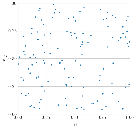
- Here we show a two dimensional projection of an IID object:
Figure 1: Uniform IID Object Projection
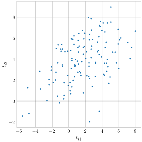
- Here we show a two dimensional projection of a Gaussian object and how
the axes returned by the
plot_projfunction can be manipulated by adding a horizontal and vertical line to denote the x and y axis respectively:
d = 2
iid = qp.IIDStdUniform(d)
iid_gaussian = qp.Gaussian(iid,mean =[2,4],covariance=[[9,4],[4,5]])
fig,ax = qp.plot_proj(iid_gaussian, n = 2**7)
ax[0,0].axvline(x=0,color= 'k',alpha=.25); #adding vertical line
ax[0,0].axhline(y=0,color= 'k',alpha=.25); #adding horizontal line
Figure 2: Gaussian IID Object Projection
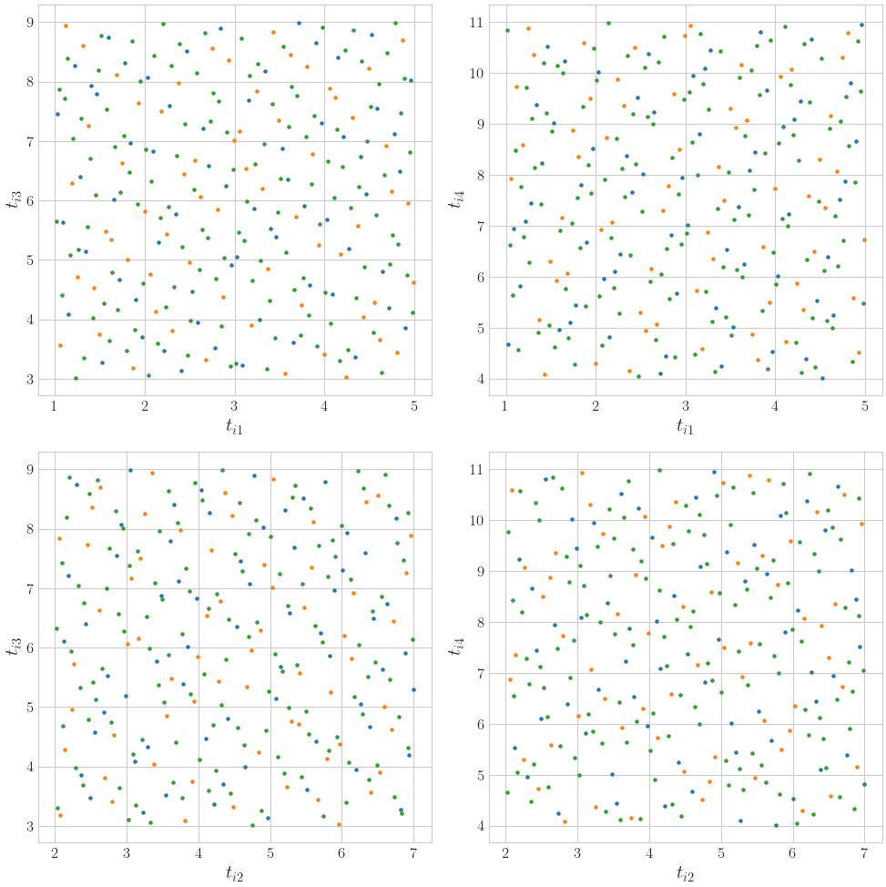
- Here we show certain specified dimensional projections, with dimensions 1 and 2 on the x axes and dimensions 3 and 4 on the y axes, of a Uniform object with successively increasing numbers of points. The initial points are in blue. The next additional points are in orange. The final additional points are in green:
d = 4
halton = qp.Halton(d)
halton_uniform = qp.Uniform(halton,lower_bound=[1,2,3,4],
upper_bound=[5,7,9,11])
fig, ax = qp.plot_proj(halton_uniform, n = [2**6, 2**7, 2**8],
d_horizontal = [1,2], d_vertical = [3,4])
Figure 3: Halton Object Projection
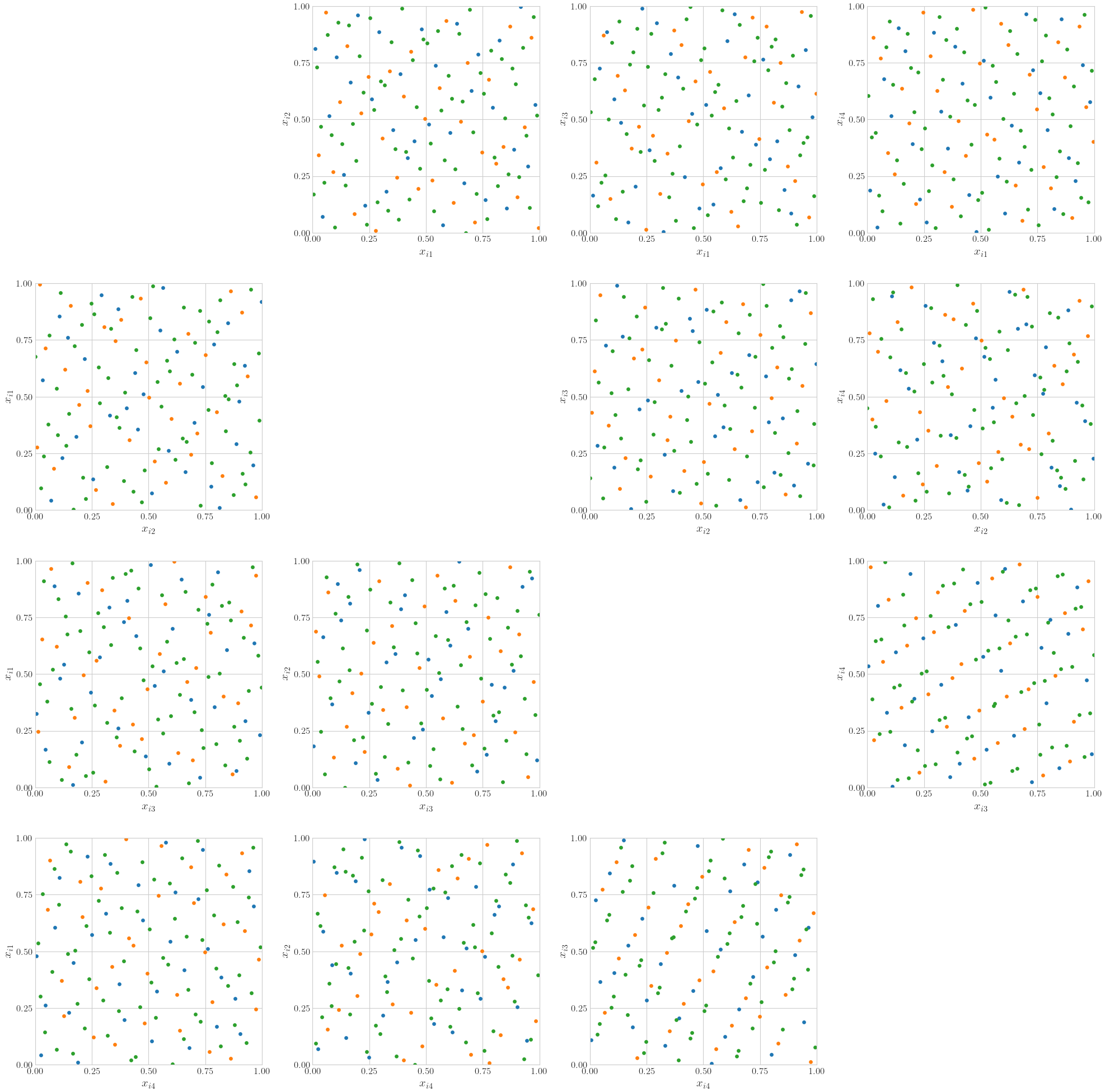
- Here we show a four dimensional projection of a Halton object with successively increasing numbers of points. The initial points are in blue. The next additional points are in orange. The final additional points are in green:
d = 4
halton = qp.Halton(d)
fig,ax = qp.plot_proj(halton, n = [2**5, 2**6, 2**7],
d_horizontal = range(d), d_vertical = range(d),
math_ind = False, marker_size = 15)
Figure 4: Halton Object Projection (More Points)
How This Function Benefits Us
In addition to making it easy to see the difference between different
Discrete Distribution and True Measure objects, this function consists of
many features that makes it user-friendly and help generate a strong and
precise visualization of the different Discrete Distribution and True
Measure objects. For instance, the extensibility feature enables us to
see how the space of the plot fills up, the marker_size parameter
helps make the samples/points bigger when plotting high-dimensional
projections, and the math_ind parameter allows the user to either input
mathematical or Python dimensions for the sampler based on one's
preference. This function could also be developed in the future to
support other distributions such as Brownian Motion.