Random Lattice Generators are Not Bad
Bocheng David Zhang
May 16, 2023
This post discusses random lattice generating vectors in QMCPy and compares mean, median, and randomly shifted lattice rules.
Generating vectors are used by lattice generators to compute point sets. Previous works [1, 2, 3, 4] commonly applied greedy component-by-component (CBC) algorithms to construct generating vectors. However, this process is dependent on weight vectors and the decay of Fourier coefficients. To this end, Takashi Goda and Pierre L'Ecuyer suggested in their work [5] that generating vectors do not require a predetermined weight vector and a measure of the decay of Fourier coefficients to reach high precision; instead, random generators can also achieve desirable results. Recently, we implemented random generating vectors into QMCPy, and the results were quite promising. This blog explores the usage of random generating vectors in QMCPy through code examples. Before that, however, we shall consider some mathematics behind generating vectors.
Mathematics of Generating Vectors
Given \(N > 2\) and generating vector \(z \in \{1,\dots,N-1\}^d\), define \(P_N := P_{N,z} := \{\boldsymbol{x}_0,\boldsymbol{x}_1,\dots, \boldsymbol{x}_{N-1}\} \subset [0,1)^d\), where
and \(\{s\} = s-\lfloor s \rfloor\) denotes the fractional part of each component. The significance of the generating vector is that it determines the point set \(P_N\).
The following are plots of lattices generated by QMCPy when \(N\) is a power of 2:
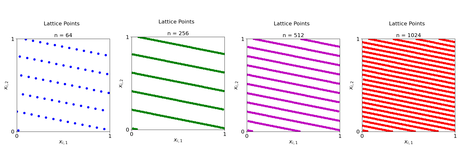
generating_vector=16 and seed=136. These plots can be conditionally reproduced in the lattice random generator notebook.While samples in [5] were produced by a prime sample size, QMCPy utilizes sample sizes that are powers of 2 due to its expectation of extensible generating vectors. The usage of the generating vector comes from quasi-Monte Carlo integration using a point set \(P_N\):
In their work, Goda and L'Ecuyer approximated \(I(f)\) by the median rule, \(\operatorname{median}(I(f;P_{N,z_1}),\dots,I(f;P_{N,z_r}))\) [5], while QMCPy utilizes mean rules, \(\operatorname{mean}(I(f;P_{N,z_1}),\dots,I(f;P_{N,z_r}))\). We performed numerical experiments in the final section to have a glimpse of the efficiency of both rules.
Code Examples
In this section, we will explore the basic features of the Lattice
class and the gen_samples method. For further documentation, see the
QMCPy Lattice documentation.
The generating vector is the core of the Lattice object. Currently,
QMCPy enables the following types of cubature schemes:
- A hard-coded \(d\)-dimensional array.
- A file that contains a hard-coded generating vector.
- A totally random generator produced by integer input.
We will focus on the recently developed third type of generating vector because it is a direct application of the mathematics discussed above.
Lattice Declaration and the gen_samples Function
A Lattice object in QMCPy requires the dimension and the generating
vector of choice. Other arguments such as randomize or seed are
optional.
The following code is a short example used to illustrate the declaration
of a Lattice object and the gen_samples function.
import qmcpy as qp
lattice = qp.Lattice(dimension=2, generating_vector=21, seed=120) # intialize the lattice
print(lattice) # print information about the lattice
print(lattice.gen_samples(n=4)) # print the first 4 points in the lattice
The output is listed below:
Lattice (AbstractLDDiscreteDistribution)
    d               2^(1)
    replications    1
    randomize       SHIFT
    gen_vec_source  random
    order           RADICAL INVERSE
    n_limit         2^(21)
    entropy         120
[[0.34548142 0.46736834]
 [0.84548142 0.96736834]
 [0.59548142 0.21736834]
 [0.09548142 0.71736834]]
Integration
To integrate in QMCPy, one needs to declare the dimension, the tolerance, a low discrepancy sequence, and the true measure used to transform the objective function to the \(d\)-dimensional unit cube. In the following example, the Gaussian measure is applied using a lattice as the low discrepancy sequence. The Keister function [6] is used as an example.
import qmcpy as qp

d = 5
tol = 1E-3

data_random = qp.CubQMCLatticeG(
    qp.Keister(
        qp.Gaussian(
            qp.Lattice(d, generating_vector=26),
            mean=0, covariance=1/2)),
    abs_tol = tol).integrate()[1]
print("Integration data from a random lattice generator:")
print(data_random)

data_default = qp.CubQMCLatticeG(
    qp.Keister(
        qp.Gaussian(
            qp.Lattice(d),
            mean=0, covariance=1/2)),
    abs_tol = tol).integrate()[1]
print("\nIntegration data from the default lattice generator:")
print(data_default)
Abbreviated output is listed below:
Integration data from a random lattice generator:
LDTransformData (AccumulateData Object)
    solution        1.136
    comb_bound_low  1.135
    comb_bound_high 1.137
    comb_flags      1
    n_total         2^(17)
    n               2^(17)
    time_integrate  0.642
Lattice (DiscreteDistribution Object)
    d               5
    dvec            [0 1 2 3 4]
    randomize       1
    order           natural
    gen_vec         [       1 29661439 12472787 51447409 58451577]
    entropy         39936265299936103070191134814877412899
    spawn_key       ()

Integration data from the default lattice generator:
LDTransformData (AccumulateData Object)
    solution        1.135
    comb_bound_low  1.134
    comb_bound_high 1.135
    comb_flags      1
    n_total         2^(17)
    n               2^(17)
    time_integrate  0.626
Lattice (DiscreteDistribution Object)
    d               5
    dvec            [0 1 2 3 4]
    randomize       1
    order           natural
    gen_vec         [     1 182667 469891 498753 110745]
    entropy         230872234427376376523997454058047592711
    spawn_key       ()
One can see that the default generator performs slightly better than the random generator, as the time to integrate is about \(0.16\) seconds lower.
Comparison Between Lattice Generators
To have a further glimpse into the performance of lattice generators, we compared the error of three types of random generators with respect to the sample size. The blue line depicts a random generator that applies the median rule \(\operatorname{median}(I(f;P_{N,z_1}),\dots,I(f;P_{N,z_r}))\); the orange line depicts a generator that applies the mean rule \(\operatorname{mean}(I(f;P_{N,z_1}),\dots,I(f;P_{N,z_r}))\); the green line is a randomly shifted hard-coded generator.
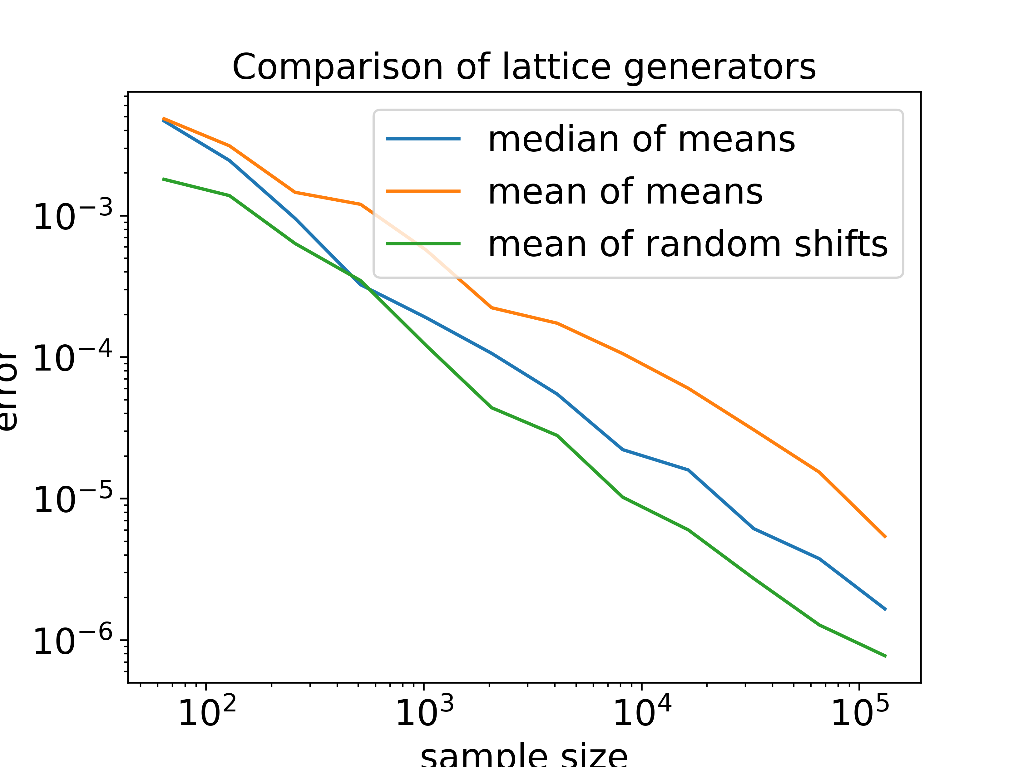
Here, we used sample sizes \(N\) ranging from \(2^6\) to \(2^{18}\) and \(r = 11\). We compared the results of integrating the 2-dimensional Keister integral over each sample size using each type of lattice generator. To reduce sampling variance, we repeated the trials \(25\) times and computed the averaged result.
As shown in the plot, the mean of random shifts (green) outperforms the random generator using median rules (blue), which in turn outperforms the random generator using mean rules (orange). These results support findings in [5]. More numerical experiments under different circumstances should be conducted before making a conclusion, but current work suggests that random lattice generators have a lot of potential.
References
- Korobov, N. M. The approximate computation of multiple integrals. Doklady Akademii Nauk SSSR 124, 1207-1210 (1959).
- Sloan, I. H. QMC integration: beating intractability by weighting the coordinate directions. In Monte Carlo and Quasi-Monte Carlo Methods 2000 (eds. Fang, K. T., Hickernell, F. J., & Niederreiter, H.) 103-123 (Springer-Verlag, Berlin, 2002).
- Kuo, F. Y. Component-by-component constructions achieve the optimal rate of convergence for multivariate integration in weighted Korobov and Sobolev spaces. Journal of Complexity 19, 301-320 (2003).
- Nuyens, D. & Cools, R. Fast component-by-component construction. In Monte Carlo and Quasi-Monte Carlo Methods 2004 (eds. Niederreiter, H. & Talay, D.) 373-387 (Springer-Verlag, Berlin, 2006).
- Goda, T. & L'Ecuyer, P. Construction-free median quasi-Monte Carlo rules for function spaces with unspecified smoothness and general weights. SIAM Journal on Scientific Computing 44, A2765-A2788 (2022). https://doi.org/10.1137/22M1473625
- Keister, B. D. Multidimensional quadrature algorithms. Computers in Physics 10, 119-122 (1996).