A QMCPy Quick Start
Aleksei Sorokin and Sou-Cheng Choi
July 6, 2020
This quick start introduces QMCPy through the Keister integration problem and shows how a discrete distribution, true measure, integrand, and stopping criterion fit together.
QMCPy is an open-source, object-oriented quasi-Monte Carlo (QMC) software framework in Python 3. It contains standardized parent classes for modeling integrands, true measures, discrete distributions, and stopping criteria. The framework is designed to help researchers and users quickly extend and experiment with new algorithmic components, validate theory, and compare proven methods in their own applications.
QMCPy can be installed with pip install qmcpy. The source code is available from the
QMCSoftware GitHub repository.
Keister Integration Problem
This quick start introduces the QMCPy workflow through the Keister function [2]. We integrate the Keister function with respect to a \(d\)-dimensional Gaussian measure:
The target integral is
Here \(\|\boldsymbol{x}\|\) is the Euclidean norm, \(\boldsymbol{I}_d\) is the \(d\)-dimensional identity matrix, and \(\Phi\) denotes the standard normal cumulative distribution function. When \(d=2\), the exact value is approximately \(\mu \approx 1.80819\).
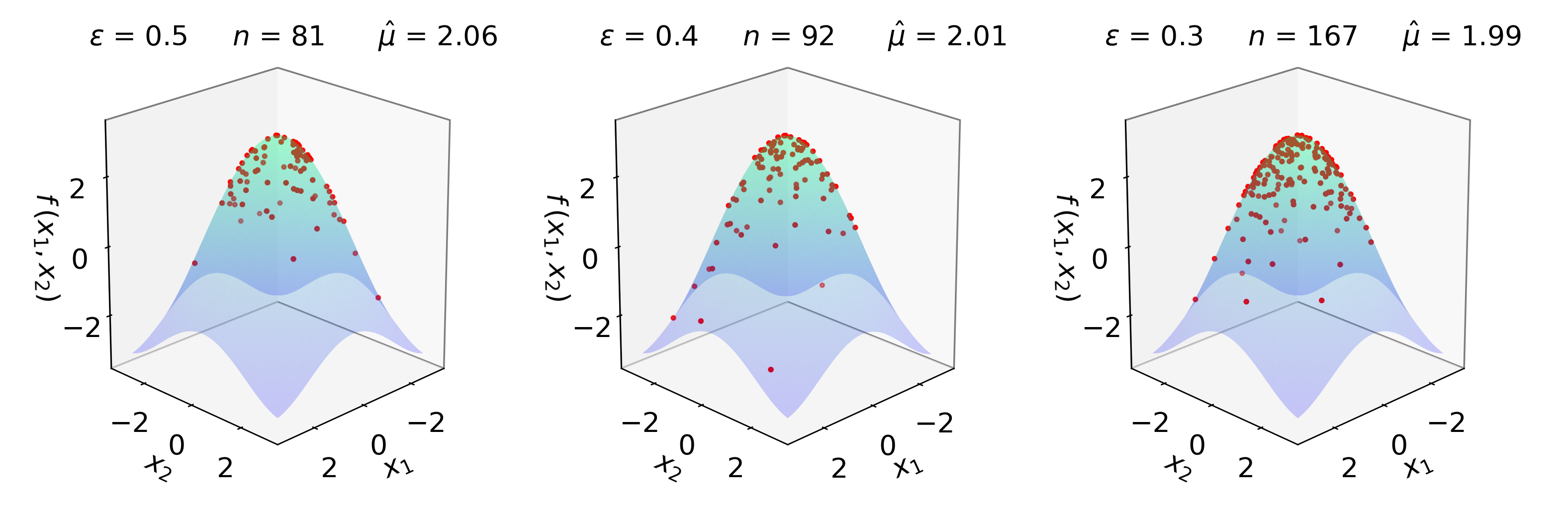
Define the Integrand
The Keister function can be implemented with NumPy:
import numpy as np

def keister(x):
    """
    x: nxd numpy ndarray with n samples d dimensions
    returns n-vector of the Keister function evaluations
    """
    d = x.shape[1]
    norm_x = np.sqrt((x**2).sum(1))
    k = np.pi**(d/2) * np.cos(norm_x)
    return k # size n vector
Set Up QMCPy Objects
In addition to the Keister integrand and Gaussian true measure, we must select a discrete distribution and a stopping criterion. The discrete distribution determines the sites at which the integrand is evaluated. The stopping criterion determines how many points are needed for the mean approximation to satisfy a user-specified error tolerance, \(\varepsilon\).
For this example, we use a lattice sequence and the corresponding lattice-based cubature stopping criterion:
import qmcpy
lattice = qmcpy.Lattice(dimension = 2, seed = 7)
gaussian = qmcpy.Gaussian(lattice, mean = 0, covariance = 1/2)
cf_keister = qmcpy.CustomFun(gaussian, g = keister)
stopping_criterion = qmcpy.CubQMCLatticeG(cf_keister, abs_tol = 1e-4)
Calling integrate on the stopping criterion returns the numerical
solution and a data object. Printing the data object provides a summary
of the integration problem:
One run gives:
Data (Data)
    solution        1.808
    comb_bound_low  1.808
    comb_bound_high 1.808
    comb_bound_diff 1.28e-04
    comb_flags      1
    n_total         2^(16)
    n               2^(16)
    time_integrate  0.017
CubQMCLatticeG (AbstractStoppingCriterion)
    abs_tol         1.00e-04
    rel_tol         0
    n_init          2^(10)
    n_limit         2^(30)
CustomFun (AbstractIntegrand)
Gaussian (AbstractTrueMeasure)
    mean            0
    covariance      2^(-1)
    decomp_type     PCA
Lattice (AbstractLDDiscreteDistribution)
    d               2^(1)
    replications    1
    randomize       SHIFT
    gen_vec_source  kuo.lattice-33002-1024-1048576.9125.txt
    order           RADICAL INVERSE
    n_limit         2^(20)
    entropy         7
This guide is a quick introduction to the QMCPy framework and syntax, not an exhaustive overview. See the searchable QMCPy documentation for more details.
References
- Choi, S.-C. T., Hickernell, F. J., McCourt, M., Rathinavel, J., & Sorokin, A. QMCPy: A quasi-Monte Carlo Python Library. https://qmcsoftware.github.io/QMCSoftware/. 2020.
- Keister, B. D. Multidimensional Quadrature Algorithms. Computers in Physics 10, 119-122. 1996.
- Oliphant, T. Guide to NumPy. Trelgol Publishing, USA, 2006.
- Hickernell, F. J., Choi, S.-C. T., Jiang, L., & Jimenez Rugama, L. A. Quasi-Monte Carlo Methods. In Wiley StatsRef: Statistics Reference Online. John Wiley & Sons, 2018.
- Jimenez Rugama, L. A. & Hickernell, F. J. Adaptive multidimensional integration based on rank-1 lattices. In Monte Carlo and Quasi-Monte Carlo Methods: MCQMC, Leuven, Belgium, April 2014, 407-422. Springer-Verlag, Berlin, 2016. arXiv:1411.1966.