Highly Efficient Geometric Brownian Motion Modeling with QMCPy
Larysa Matiukha, Aleksei Sorokin, and Sou-Cheng Choi
October 22, 2025
This post demonstrates how QMCPy can generate and analyze Geometric Brownian Motion paths efficiently for simulation and finance workflows.
Example implementation of GBM using QMCPy
Install the required Python packages:
Generate 16 paths on \([0,1]\) with QMCPy's sampler (\(S_0=1\), \(\mu=0.05\), \(\sigma^2=0.2\)) and plot five:
import numpy as np
import matplotlib.pyplot as plt
import qmcpy as qp

sampler = qp.Lattice(252, seed=42)  # daily steps for 1 year
gbm = qp.GeometricBrownianMotion(
    sampler, t_final=1, initial_value=1, drift=0.05, diffusion=0.2
)
paths = gbm.gen_samples(16)
t = np.linspace(0, 1.0, paths.shape[1])
plt.plot(t, paths[:5].T, alpha=0.8)
plt.xlabel("$t$")
plt.ylabel("$S_t$")
plt.title("GBM paths")
plt.show()
Introduction
In this blog, we demonstrate how to simulate and analyze a geometric Brownian motion (GBM) process using QMCPy in Python. GBM is widely used in finance to model stock prices and other assets. We will walk through key code snippets, plots, and insights. The numerical results can be reproduced using the GBM demo notebook.
GBM is a continuous stochastic process in which the natural logarithm of its values follows a Brownian motion (BM) [1]. Mathematically, it can be defined as follows:
where
- \(S_0\) is the initial value,
- \(\mu\) is a drift coefficient,
- \(\sigma\) is the volatility (note: QMCPy uses diffusion \(= \sigma^2\)),
- \(W_t\) is a standard BM.
At any time \(0 < t \le T\), where \(0\) and \(T\) represent the beginning and end time of the process, \(S_t\) follows a log-normal distribution with expected value and variance as follows (see Section 3.2 in [1]):
- \(E[S_t] = S_0 e^{\mu t}\),
- \(\operatorname{Var}[S_t] = S_0^2 e^{2\mu t}(e^{\sigma^2 t} - 1)\),
- \(\operatorname{Cov}(S_{t_i}, S_{t_j}) = S_0^2 e^{\mu(t_i + t_j)} \left(e^{\sigma^2 \min(t_i, t_j)} - 1\right)\).
GBM is commonly used to model stock prices driving option payoffs in derivatives pricing [2, 3].
GBM Objects in QMCPy
GBM in QMCPy inherits from BrownianMotion [4, 5]. We can instantiate a
GBM class and generate sample paths to see the class in action:
import qmcpy as qp

qp_gbm = qp.GeometricBrownianMotion(qp.Lattice(2, seed=42))
qp_gbm.gen_samples(n=4)
The output shows 4 sample paths evaluated at 2 time points, yielding a \((4 \times 2)\) array where rows represent paths and columns represent time steps:
Log-Normality Property
The log-normal property is fundamental in financial modeling because it ensures asset prices remain strictly positive while allowing for unlimited upside potential. This property makes GBM the cornerstone of the Black-Scholes model and many derivative pricing frameworks.
To validate theoretical properties, we generate \(2^{12} = 4096\) paths
over 5 time steps and compare empirical moments with theoretical values.
The theoretical values match the last values captured in
qp_gbm.mean_gbm and qp_gbm.covariance_gbm for the final time point.
# Generate GBM samples for theoretical validation
import qmcpy as qp
import numpy as np

S0, mu, sigma, T, n_samples = 100.0, 0.05, 0.20, 1.0, 2**12
diffusion = sigma**2
sampler = qp.Lattice(5, seed=42)
qp_gbm = qp.GeometricBrownianMotion(
    sampler, t_final=T, initial_value=S0, drift=mu, diffusion=diffusion
)
paths = qp_gbm.gen_samples(n_samples)
S_T = paths[:, -1]  # Final values only

# Calculate theoretical vs empirical sample moments
theo_mean = S0 * np.exp(mu * T)
theo_var = S0**2 * np.exp(2 * mu * T) * (np.exp(diffusion * T) - 1)
qp_emp_mean = np.mean(S_T)
qp_emp_var = np.var(S_T, ddof=1)
print(f"Mean: {qp_emp_mean:.3f} (theoretical: {theo_mean:.3f})")
print(f"Variance: {qp_emp_var:.3f} (theoretical: {theo_var:.3f})")
qp_gbm
| Statistic | Value |
|---|---|
| Sample Mean | 105.127 (Theoretical: 105.127) |
| Sample Variance | 449.776 (Theoretical: 451.029) |
| Time Vector | \([0.2,\; 0.4,\; 0.6,\; 0.8,\; 1.0]\) |
| Drift (\(\mu\)) | 0.05 |
| Diffusion (\(\sigma^2\)) | 0.040 |
| Mean | \([101.005,\; 102.020,\; 103.045,\; 104.081,\; 105.127]\) |
| Decomposition Type | PCA |
| Covariance Matrix | \(\left[\begin{array}{rrrrr} 81.943 & 82.767 & 83.599 & 84.439 & 85.288 \\ 82.767 & 167.869 & 169.556 & 171.260 & 172.981 \\ 83.599 & 169.556 & 257.923 & 260.516 & 263.134 \\ 84.439 & 171.260 & 260.516 & 352.258 & 355.798 \\ 85.288 & 172.981 & 263.134 & 355.798 & 451.029 \end{array}\right]\) |
GBM vs BM
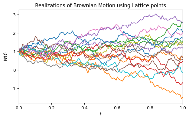
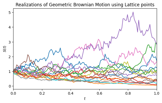
Below we compare BM and GBM using the same parameters:
drift = 0, diffusion = 1, and initial_value = 1. The driftless BM
paths should fluctuate symmetrically around the initial value (\(y = 1\))
and can take negative values, while the GBM paths remain strictly
positive.
n = 16
sampler = qp.Lattice(2**7, seed=42)
plot_paths("BM", sampler, t_final=1, initial_value=1, drift=0, diffusion=1, n=n)
plot_paths("GBM", sampler, t_final=1, initial_value=1, drift=0, diffusion=1, n=n)
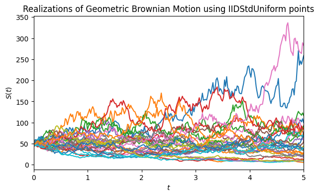
Next, we demonstrate how easily one can swap samplers or change parameters in QMCPy. For example, to model a stock price with initial value \(S_0=50\), drift \(\mu=0.1\), and volatility \(\sigma=\sqrt{0.2}\) over a 5-year horizon using IID sampling:
gbm_iid = plot_paths(
    "GBM",
    qp.IIDStdUniform(2**8, seed=42),
    t_final=5,
    initial_value=50,
    drift=0.1,
    diffusion=0.2,
    n=32,
)
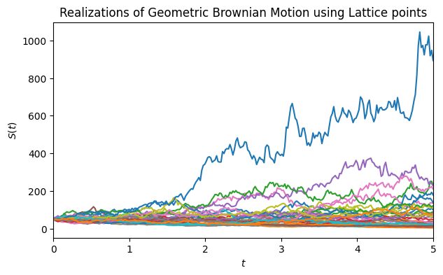
We can also use a low-discrepancy lattice sampler with the same parameters:
gbm_lattice = plot_paths(
    "GBM",
    qp.Lattice(2**8, seed=42),
    t_final=5,
    initial_value=50,
    drift=0.1,
    diffusion=0.2,
    n=32,
)
The generated sample paths are plotted below. The four panels show, respectively:
- BM with lattice sampler (\(T=1\), \(S_0=1\), \(\mu=0\), \(\sigma^2=1\), 16 paths),
- GBM with lattice sampler (\(T=1\), \(S_0=1\), \(\mu=0\), \(\sigma^2=1\), 16 paths),
- GBM with IID sampler (\(T=5\), \(S_0=50\), \(\mu=0.1\), \(\sigma^2=0.2\), 32 paths),
- GBM with lattice sampler (\(T=5\), \(S_0=50\), \(\mu=0.1\), \(\sigma^2=0.2\), 32 paths).
QuantLib vs QMCPy Comparison
In this section, we compare QMCPy's GeometricBrownianMotion
implementation with the industry-standard QuantLib library [6] to
validate its accuracy and performance. The numerical results are
summarized in the following table.
Both libraries produce statistically equivalent GBM simulations that match theoretical values. QMCPy typically runs 1.5 to 2 times faster due to vectorized operations, lazy loading, and optimized memory management. More importantly, it demonstrates superior numerical accuracy (lower mean absolute errors) with Sobol, lattice, and Halton samplers, making it useful for research and high-performance applications. QuantLib remains the industry standard for production systems that require comprehensive support for financial modeling and risk management.
| Method | Sampler | Mean | Std Dev | Mean Absolute Error | Std Dev Error | Mean Time (s) | Std Dev (s) | Speedup |
|---|---|---|---|---|---|---|---|---|
| QuantLib | Sobol | 100.88887227 | 0.00000000 | 4.23823737 | 21.23743882 | 0.00009037 | 0.00000000 | - |
| QMCPy | Sobol | 103.66893699 | 1.17417404 | 1.45817264 | 20.06326479 | 0.00143112 | 0.00000000 | 0.08401794 |
import QuantLib as ql
import numpy as np


def generate_quantlib_paths(
    initial_value: float,
    mu: float,
    sigma: float,
    maturity: float,
    n_steps: int,
    n_paths: int,
    sampler_type: str = "IIDStdUniform",
    seed: int = 7,
) -> tuple:
    """
    Generate Geometric Brownian Motion paths using QuantLib.

    Args:
        initial_value: Initial value of the GBM process (S_0)
        mu: Drift parameter
        sigma: Volatility parameter (note: NOT diffusion coefficient)
        maturity: Final time T
        n_steps: Number of discretization time steps
        n_paths: Number of paths to generate
        sampler_type: Type of sampler ('IIDStdUniform' or 'Sobol')
        seed: Random seed for reproducibility

    Returns:
        tuple: (paths, gbm) where paths has shape (n_paths, n_steps+1)
               (includes initial value at t=0) and gbm is the
               GeometricBrownianMotionProcess object

    Raises:
        ValueError: If sampler_type is not 'IIDStdUniform' or 'Sobol'
    """
    gbm = ql.GeometricBrownianMotionProcess(initial_value, mu, sigma)
    times = ql.TimeGrid(maturity, n_steps)
    dimension = n_steps
    if sampler_type == "IIDStdUniform":
        uniform_rng = ql.UniformRandomGenerator(seed)
        sequence_gen = ql.GaussianRandomSequenceGenerator(
            ql.UniformRandomSequenceGenerator(n_steps, uniform_rng)
        )
        path_gen = ql.GaussianPathGenerator(gbm, maturity, n_steps, sequence_gen, False)
        paths = np.zeros((n_paths, n_steps + 1))
        for i in range(n_paths):
            sample_path = path_gen.next().value()
            paths[i, :] = np.array([sample_path[j] for j in range(n_steps + 1)])
        return paths, gbm
    elif sampler_type == "Sobol":
        uniform_rsg = ql.UniformLowDiscrepancySequenceGenerator(dimension, seed)
        sequence_gen = ql.GaussianLowDiscrepancySequenceGenerator(uniform_rsg)
        path_gen = ql.GaussianSobolMultiPathGenerator(
            gbm, list(times), sequence_gen, False
        )
        paths = np.zeros((n_paths, n_steps + 1))
        paths[:, 0] = initial_value  # Set initial value
        for i in range(n_paths):
            sample_path = path_gen.next().value()
            # For 1D process, get the first (and only) path
            path_values = sample_path[0]
            paths[i, :] = np.array([path_values[j] for j in range(n_steps + 1)])
        return paths, gbm
    else:
        raise ValueError(
            f"Unsupported sampler type: {sampler_type}.  Use 'IIDStdUniform' or 'Sobol'"
        )
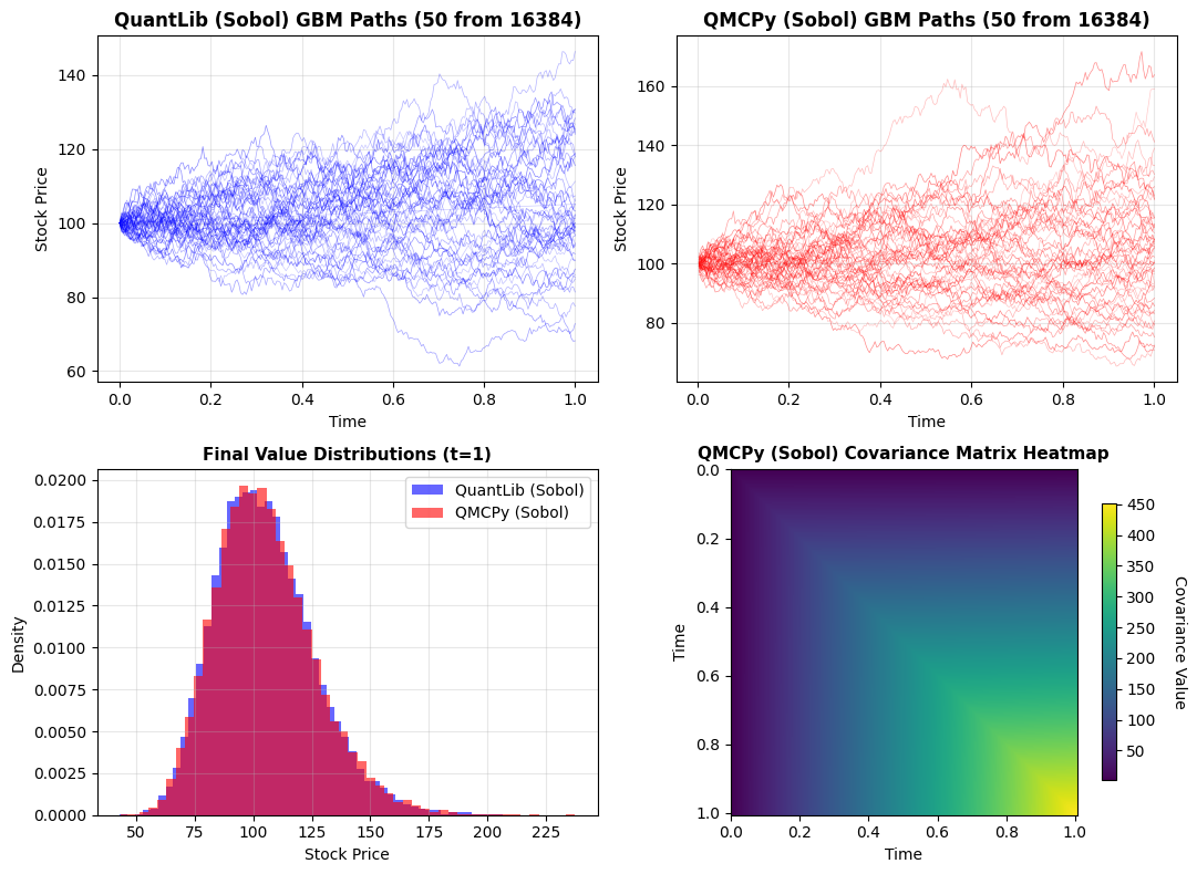
In the next figure, the top row shows sample paths: QMCPy on the left and QuantLib on the right. The bottom-left panel overlays the marginal distribution at \(t=1\), where both libraries yield nearly identical shapes with means and standard deviations matching the table above. The bottom-right panel is a QMCPy covariance heatmap with time 0 at the top of the \(y\)-axis; the variance increases along the diagonal with time and the off-diagonal structure follows \(\min(t_i,t_j)\), consistent with the analytic form and the numerical matrix above.
The evaluation of computational efficiency was done by creating
comprehensive performance benchmarks comparing QMCPy and QuantLib across
two key scaling dimensions. The benchmarks were performed using the
perfplot library, which automatically handles warm-up, multiple runs,
and statistical analysis to ensure reliable timing measurements.
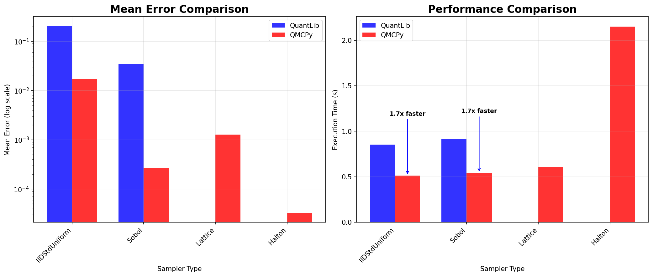
The following figure presents the results of our performance analysis. The left panel shows how execution time scales with the number of time steps while keeping the number of paths fixed at 4,096. Both libraries exhibit approximately linear scaling, but QMCPy demonstrates superior performance at smaller time step counts, with QuantLib becoming more competitive as the number of time steps increases. The right panel examines scaling behavior with respect to the number of paths while fixing the time steps at 252, representing a typical trading year. Here, QMCPy maintains a consistent performance advantage across all path counts, with the gap becoming more pronounced at higher path numbers. This performance difference is particularly relevant for Monte Carlo applications that require large numbers of simulation paths for accurate estimation.
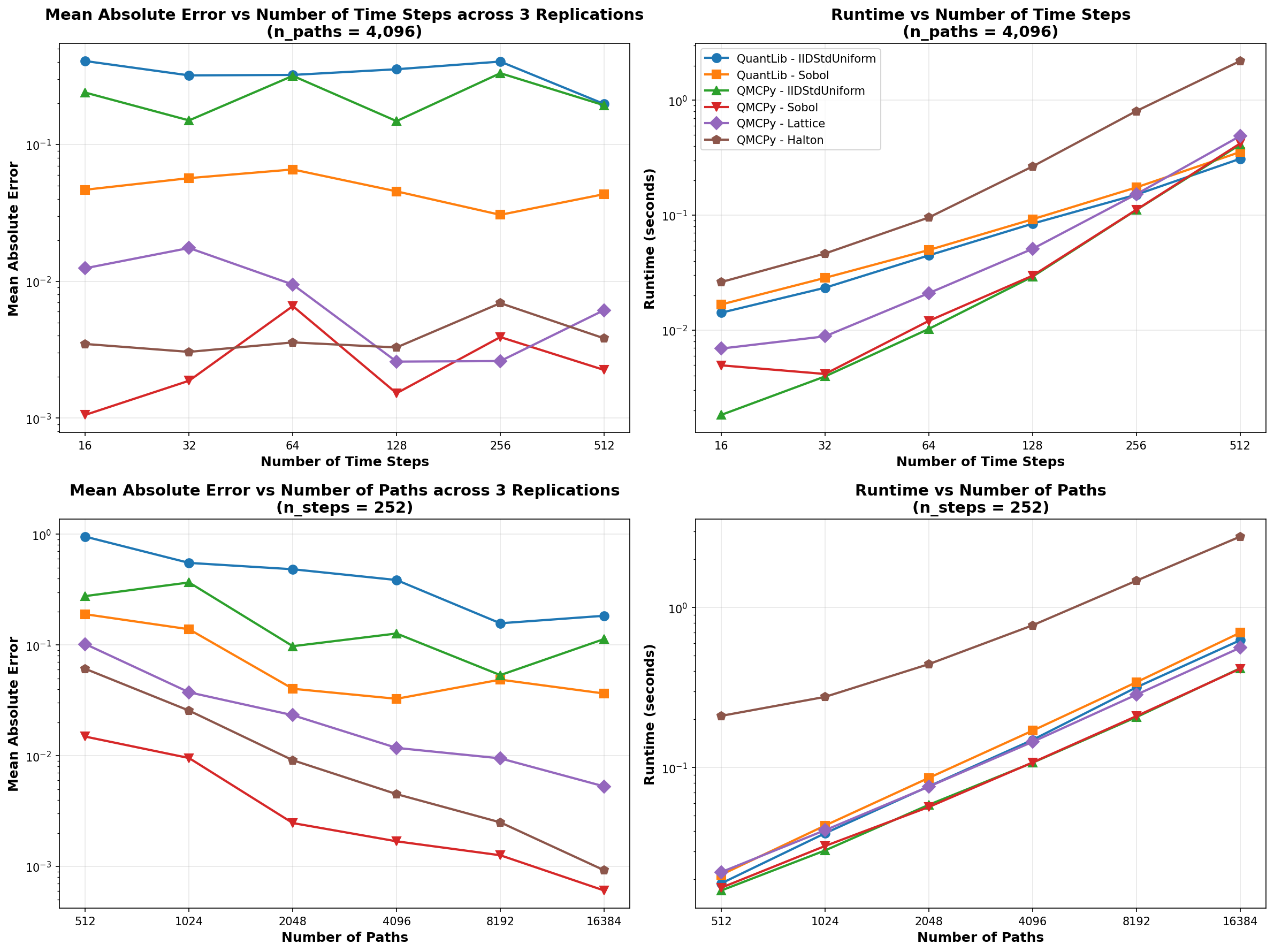
To further validate these performance findings, we conducted an extended parameter sweep analysis across a broader range of configurations. The next figure presents the comprehensive results of this analysis, systematically examining performance across varying time steps and path counts.
- Regarding accuracy, QMCPy's Sobol sampler generally achieves the lowest mean absolute error (MAE), particularly when a larger number of paths are used, reaching errors below \(10^{-3}\). The lattice sampler also provides competitive accuracy, especially with higher path counts. While QuantLib's standard uniform IID sampler yields slightly lower MAE for a larger number of paths compared to QMCPy's IID sampler, it is notably slower.
- Regarding speed, low-discrepancy samplers like Sobol, lattice, and Halton demonstrate superior convergence rates with increasing path counts compared to IID methods. With QMCPy, Sobol and lattice samplers offer the best speed-accuracy trade-off. QuantLib achieves comparable runtime to QMCPy's faster samplers, but without the accuracy benefits. The Halton sampler, while yielding the most accurate results, incurs significantly higher computational costs. These results highlight QMCPy's quasi-Monte Carlo methods as particularly well-suited for applications requiring high accuracy, with Sobol and lattice samplers providing an optimal balance of speed and precision for most practical scenarios.
Internals
The GeometricBrownianMotion class in QMCPy is engineered for speed,
robustness, and mathematical correctness. Its design leverages
object-oriented inheritance and vectorized operations, resulting in both
flexibility and high performance. GeometricBrownianMotion inherits
from BrownianMotion, which itself inherits from Gaussian. This
layered design allows the GBM class to reuse and extend efficient
implementations for Gaussian random vectors and BM increments. The
constructor rigorously checks input parameters (e.g., positivity of
initial value and diffusion, valid decomposition type), ensuring
mathematical integrity and preventing run-time errors.
The class uses vectorized NumPy operations to generate entire arrays of GBM paths in a single call, minimizing Python loops and maximizing computational throughput. Sample generation proceeds in two stages:
- The parent class
BrownianMotiongenerates standard BM sample paths using the specified sampler (e.g., low-discrepancy lattice, IID uniform), with drift and diffusion handled in the mean and covariance structure. - The GBM class transforms the BM samples via the exponential mapping above, performed in a fully vectorized fashion, ensuring that thousands of paths can be efficiently simulated.
The class computes and stores the theoretical mean and covariance matrices for GBM at initialization, which can be used for validation and theoretical comparisons. Both mean and covariance are calculated using analytical formulas, leveraging NumPy broadcasting for efficient computations. Briefly, broadcasting in NumPy allows arithmetic operations between arrays of different shapes by automatically expanding the smaller array to match the shape of the larger array.
The Gaussian and BM classes both implement Cholesky and PCA factorization of the covariance matrix
respectively. In the Cholesky method, one computes the lower-triangular \(L=\operatorname{chol}(\Sigma)\) and obtains correlated increments via \(X=LZ\), where \(Z\sim\mathcal{N}(0,I)\). In the PCA approach, one first diagonalizes \(\Sigma=PDP^\top\), then forms \(X = P D^{1/2} Z\). By default PCA is used for its superior numerical stability in high dimensions and slightly lower cost when many eigenvalues are near zero. These correlated normals feed directly into the GBM update
ensuring that the simulated paths respect the intended covariance structure and remain strictly positive, with strict-positivity checks raising warnings or errors if violated.
Conclusions and Future Work
This blog demonstrates that QMCPy's quasi-Monte Carlo implementations provide significant advantages over traditional Monte Carlo methods for modeling geometric Brownian motion. QMCPy's approach combines superior numerical accuracy with enhanced computational efficiency, making it particularly well-suited for high-performance financial modeling applications.
In the future, we aim to investigate ways to improve the runtime of the Halton sampler. For example, we may consider starting with Halton sampling points for high accuracy in early iterations, then switch to Sobol for faster convergence as sample size increases. It would also be interesting to experiment with ensemble sampling by running multiple samplers in parallel and combine the results using weighted averaging based on their relative accuracies.
Takeaways
To the best of our knowledge, this blog presents the first publicly available benchmark comparing QuantLib and QMCPy for Geometric Brownian Motion simulations. Key takeaways include:
- Theoretical Validation: QMCPy's GBM implementation correctly preserves log-normality and matches theoretical moments, providing reliable foundations for financial modeling applications.
- QMC Advantage: Quasi-Monte Carlo methods (Sobol, lattice, Halton) demonstrate superior convergence and accuracy compared to traditional Monte Carlo, with Halton achieving the lowest mean error and Sobol providing consistent performance across scenarios.
- Flexibility and Ease of Use: Change one argument in QMCPy to swap samplers or covariance decompositions, enabling rapid experimentation and method comparison.
- Performance: Vectorized operations and optimized memory management produce 1.5-2x faster path generation than QuantLib.
- Robustness: Superior numerical stability through PCA decomposition and comprehensive error handling make QMCPy suitable for both research and practical financial and scientific applications.
References
- Glasserman, P. Monte Carlo Methods in Financial Engineering. Springer-Verlag, New York, 2004.
- Hull, J. Options, Futures, and Other Derivatives (10th ed.). Pearson, 2017.
- Ross, S. M. Introduction to Probability Models (11th ed.). Academic Press, 2014.
- Choi, S.-C. T., Hickernell, F. J., Jagadeeswaran, R., McCourt, M. J., & Sorokin, A. G. Quasi-Monte Carlo Software. In A. Keller (Ed.), Monte Carlo and Quasi-Monte Carlo Methods, 2022.
- Choi, S.-C. T., Hickernell, F., McCourt, M., & Sorokin, A. QMCPy: A quasi-Monte Carlo Python Library. https://qmcsoftware.github.io/QMCSoftware/. 2020.
- The QuantLib contributors. QuantLib: A free/open-source library for quantitative finance. Version 1.38. DOI: 10.5281/zenodo.1440997. 2003--2025. https://www.quantlib.org.
Acknowledgments
The authors thank Fred Hickernell, Joshua Jay Herman and Jiangrui Kang for their insightful feedback and help with the blog post.